SDE 몬테카를로 분포

이 notebook은 pyna에서 SDE를 실제로 어떻게 쓰는지 보여 주는 사례입니다. 모델의 책임 범위와 단일 경로의 기하 표현에는 pyna의 SDE 클래스를 사용하고, 분포 추정에는 벡터화된 NumPy ensemble을 사용합니다.

이 notebook은 문서 게시 전에 로컬에서 미리 실행해 둡니다. 저장된 출력은 GitHub Pages에서 Sphinx/nbsphinx가 그대로 렌더링하므로, 문서 workflow가 반복적인 몬테카를로 샘플링에 CI CPU 시간을 쓰지 않아도 됩니다.

%matplotlib inline
from matplotlib_inline.backend_inline import set_matplotlib_formats
set_matplotlib_formats('svg')

import numpy as np
import matplotlib.pyplot as plt

from pyna.dynamics import BrownianMotion, GeometricBrownianMotion, ItoSDE

plt.rcParams.update({
    "figure.figsize": (10, 4),
    "axes.grid": True,
    "axes.spines.top": False,
    "axes.spines.right": False,
})

rng = np.random.default_rng(20260701)
print("rng seed = 20260701")

rng seed = 20260701

브라운 운동: 종단 분포

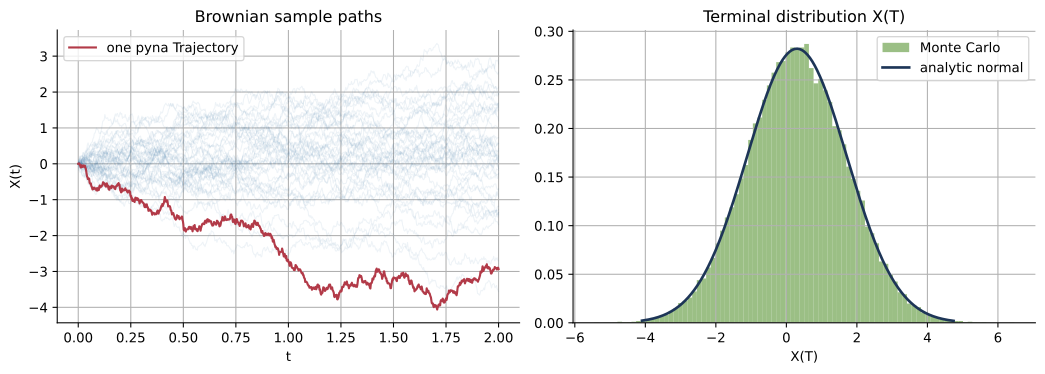
브라운 운동의 단일 realization은 하나의 Trajectory입니다. 큰 ensemble은 확률분포를 추정합니다. 브라운 운동의 종단 분포는 해석적으로 알려져 있으므로, 몬테카를로 코드의 회귀 검증에 유용합니다.

bm = BrownianMotion(dim=1, diffusion=1.0, drift=[0.15])
single_path = bm.euler_maruyama([0.0], (0.0, 2.0), dt=0.002, rng=7)

n_paths = 60_000
n_steps = 600
T = 2.0
dt = T / n_steps

increments = np.sqrt(dt) * rng.normal(size=(n_paths, n_steps))
terminal = bm.drift_vector[0] * T + increments.sum(axis=1)

times = np.linspace(0.0, T, n_steps + 1)
fan_count = 40
fan_paths = np.empty((fan_count, n_steps + 1))
fan_paths[:, 0] = 0.0
fan_paths[:, 1:] = bm.drift_vector[0] * times[1:] + np.cumsum(increments[:fan_count], axis=1)

analytic_mean = bm.mean([0.0], T)[0]
analytic_var = bm.variance(T)[0]
empirical_mean = float(np.mean(terminal))
empirical_var = float(np.var(terminal, ddof=1))

x_grid = np.linspace(np.quantile(terminal, 0.001), np.quantile(terminal, 0.999), 400)
pdf = np.exp(-0.5 * (x_grid - analytic_mean) ** 2 / analytic_var) / np.sqrt(2 * np.pi * analytic_var)

fig, axes = plt.subplots(1, 2, figsize=(11, 4))
axes[0].plot(times, fan_paths.T, color="#2f6f9f", alpha=0.08, linewidth=0.8)
axes[0].plot(single_path.t, single_path.y[:, 0], color="#b23a48", linewidth=1.6, label="one pyna Trajectory")
axes[0].set_title("Brownian sample paths")
axes[0].set_xlabel("t")
axes[0].set_ylabel("X(t)")
axes[0].legend(loc="upper left")

axes[1].hist(terminal, bins=90, density=True, color="#7aa95c", alpha=0.75, label="Monte Carlo")
axes[1].plot(x_grid, pdf, color="#1d3557", linewidth=2.0, label="analytic normal")
axes[1].set_title("Terminal distribution X(T)")
axes[1].set_xlabel("X(T)")
axes[1].legend()
plt.tight_layout()

print(f"paths = {n_paths:,}, steps = {n_steps}, T = {T}")
print(f"mean: empirical {empirical_mean:.5f}, analytic {analytic_mean:.5f}, abs error {abs(empirical_mean - analytic_mean):.5f}")
print(f"var : empirical {empirical_var:.5f}, analytic {analytic_var:.5f}, abs error {abs(empirical_var - analytic_var):.5f}")

paths = 60,000, steps = 600, T = 2.0
mean: empirical 0.29974, analytic 0.30000, abs error 0.00026
var : empirical 2.00725, analytic 2.00000, abs error 0.00725

Ornstein-Uhlenbeck 과정: 정상 법칙으로의 접근

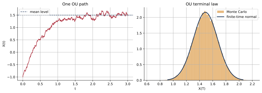
OU 과정은 평균회귀를 설명하는 간결한 교육용 모델입니다. 사용자가 정의한 drift와 diffusion을 갖는 사용자 정의 ItoSDE도 함께 보여 줍니다. 몬테카를로 ensemble은 유한 시간 정규분포와 정상 분산을 확인합니다.

theta = 1.8
mean_level = 1.5
sigma = 0.35
x0 = -1.0
T = 3.0
n_steps = 1200
dt = T / n_steps
n_paths = 80_000

ou = ItoSDE(
    drift=lambda x, t: theta * (mean_level - x),
    diffusion=lambda x, t: np.array([sigma]),
    dim=1,
    brownian_dim=1,
    coordinate_names=("x",),
    label="Ornstein-Uhlenbeck",
)
ou_path = ou.euler_maruyama([x0], (0.0, T), dt=dt, rng=11)

x = np.full(n_paths, x0, dtype=float)
sqrt_dt_sigma = sigma * np.sqrt(dt)
for _ in range(n_steps):
    x += theta * (mean_level - x) * dt + sqrt_dt_sigma * rng.normal(size=n_paths)

analytic_mean = mean_level + (x0 - mean_level) * np.exp(-theta * T)
analytic_var = sigma**2 / (2 * theta) * (1 - np.exp(-2 * theta * T))
stationary_var = sigma**2 / (2 * theta)
empirical_mean = float(np.mean(x))
empirical_var = float(np.var(x, ddof=1))

grid = np.linspace(np.quantile(x, 0.001), np.quantile(x, 0.999), 400)
pdf = np.exp(-0.5 * (grid - analytic_mean) ** 2 / analytic_var) / np.sqrt(2 * np.pi * analytic_var)

fig, axes = plt.subplots(1, 2, figsize=(11, 4))
axes[0].plot(ou_path.t, ou_path.y[:, 0], color="#b23a48", linewidth=1.4)
axes[0].axhline(mean_level, color="#1d3557", linestyle="--", linewidth=1.2, label="mean level")
axes[0].set_title("One OU path")
axes[0].set_xlabel("t")
axes[0].set_ylabel("X(t)")
axes[0].legend()

axes[1].hist(x, bins=90, density=True, color="#e0a458", alpha=0.76, label="Monte Carlo")
axes[1].plot(grid, pdf, color="#1d3557", linewidth=2.0, label="finite-time normal")
axes[1].set_title("OU terminal law")
axes[1].set_xlabel("X(T)")
axes[1].legend()
plt.tight_layout()

print(f"paths = {n_paths:,}, steps = {n_steps}, T = {T}")
print(f"mean: empirical {empirical_mean:.5f}, analytic {analytic_mean:.5f}, abs error {abs(empirical_mean - analytic_mean):.5f}")
print(f"var : empirical {empirical_var:.5f}, finite-time {analytic_var:.5f}, stationary {stationary_var:.5f}")

paths = 80,000, steps = 1200, T = 3.0
mean: empirical 1.48901, analytic 1.48871, abs error 0.00030
var : empirical 0.03427, finite-time 0.03403, stationary 0.03403

기하 브라운 운동: 주식형 장기 거동

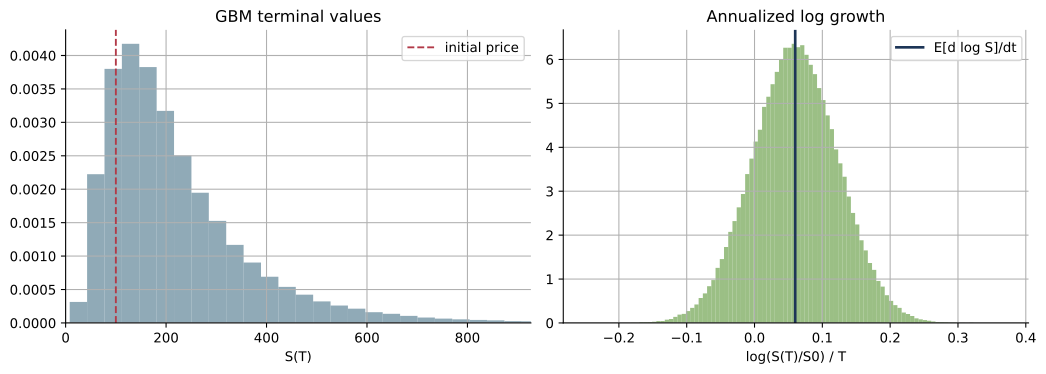
기하 브라운 운동은 곱셈 잡음을 설명하기 위한 단순화된 교육용 모델입니다. 로그 성장률을 설명하는 데 유용하지만, 매매 권고나 현실적인 시장 시뮬레이터는 아닙니다.

gbm = GeometricBrownianMotion(mu=[0.08], sigma=[0.20])
S0 = 100.0
T = 10.0
n_paths = 250_000

z = rng.normal(size=n_paths)
log_growth_rate = gbm.expected_log_growth()[0]
log_terminal = np.log(S0) + log_growth_rate * T + gbm.sigma[0] * np.sqrt(T) * z
terminal = np.exp(log_terminal)
annualized_log_returns = np.log(terminal / S0) / T

analytic_mean = gbm.mean([S0], T)[0]
empirical_mean = float(np.mean(terminal))
prob_loss = float(np.mean(terminal < S0))
quantiles = np.quantile(terminal, [0.05, 0.25, 0.50, 0.75, 0.95])

fig, axes = plt.subplots(1, 2, figsize=(11, 4))
axes[0].hist(terminal, bins=120, density=True, color="#6b8e9f", alpha=0.75)
axes[0].axvline(S0, color="#b23a48", linestyle="--", linewidth=1.4, label="initial price")
axes[0].set_title("GBM terminal values")
axes[0].set_xlabel("S(T)")
axes[0].set_xlim(0, np.quantile(terminal, 0.995))
axes[0].legend()

axes[1].hist(annualized_log_returns, bins=100, density=True, color="#7aa95c", alpha=0.75)
axes[1].axvline(log_growth_rate, color="#1d3557", linewidth=2.0, label="E[d log S]/dt")
axes[1].set_title("Annualized log growth")
axes[1].set_xlabel("log(S(T)/S0) / T")
axes[1].legend()
plt.tight_layout()

print(f"paths = {n_paths:,}, horizon = {T:g} years")
print(f"expected log growth = {log_growth_rate:.4f} per year")
print(f"mean terminal: empirical {empirical_mean:.2f}, analytic {analytic_mean:.2f}")
print(f"P[S(T) < S0] = {prob_loss:.3f}")
print("terminal quantiles 5/25/50/75/95% =", np.round(quantiles, 2))

paths = 250,000, horizon = 10 years
expected log growth = 0.0600 per year
mean terminal: empirical 222.55, analytic 222.55
P[S(T) < S0] = 0.171
terminal quantiles 5/25/50/75/95% = [ 64.56 119.13 182.27 279.15 516.16]

이 사례가 검증하는 것

• pyna의 SDE 모델은 재현 가능한 단일 경로 Trajectory 객체를 만든다.

• 브라운 운동과 OU 과정의 경험적 종단 법칙은 몬테카를로 오차 범위 안에서 해석적 평균 및 분산과 일치한다.

• GBM은 산술평균 성장과 장시간 로그 성장의 차이를 드러낸다.

운영 규모의 몬테카를로 계산에서는 모델의 책임 범위를 pyna 안에 두고, ensemble kernel은 벡터화·병렬화 또는 accelerator 기반 구현으로 옮기는 것이 좋습니다. 기하학적 주장이 명시적이고 수치적으로 정당화되지 않는 한 ensemble을 Cycle, Tube, IslandChain으로 승격하지 마십시오.