RMP Stellarator Resonance Analysis#
This notebook is the main public workflow for analytic stellarator resonance geometry. It folds two formerly separate text-only tutorials into one visual computation:
Build an analytic stellarator equilibrium and trace Poincare sections.
Compute resonant RMP Fourier components and their analytic X/O fixed points.
Promote raw section points into geometry: crossings, fixed-point markers, resonant surfaces, O-point island-width bars, local stable branches, and coordinate overlays.
Compare unperturbed and perturbed sections with a PEST-style grid.
Summarize island widths, Chirikov overlap, and the \((m,n)\) spectrum.
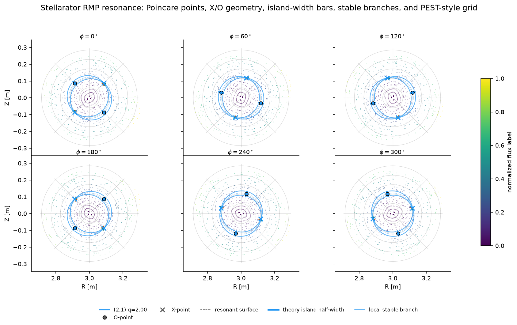
Produce a modern multi-section figure using
pyna.plothelpers.
The notebook is designed to be executed locally before publishing the docs. GitHub Pages renders the saved outputs rather than recomputing field-line traces.
[SETUP] Imports and publication style#
[1]:
import sys
import json
import pathlib
import numpy as np
import matplotlib
import matplotlib.pyplot as plt
from matplotlib.colors import Normalize

PROJECT_ROOT = None
for candidate in [pathlib.Path.cwd(), *pathlib.Path.cwd().parents]:
    if (candidate / 'pyna').is_dir() and (candidate / 'pyproject.toml').exists():
        PROJECT_ROOT = candidate
        break
if PROJECT_ROOT is not None and str(PROJECT_ROOT) not in sys.path:
    sys.path.insert(0, str(PROJECT_ROOT))

%matplotlib inline
from matplotlib_inline.backend_inline import set_matplotlib_formats
set_matplotlib_formats('png')

plt.rcParams.update({
    'font.family': 'DejaVu Sans',
    'font.size': 9,
    'axes.labelsize': 9,
    'axes.titlesize': 10,
    'figure.dpi': 150,
    'text.usetex': False,
    'axes.linewidth': 0.75,
    'axes.spines.top': False,
    'axes.spines.right': False,
    'figure.facecolor': 'white',
    'axes.facecolor': 'white',
})

from pyna.toroidal.equilibrium.stellarator import simple_stellarator
from pyna.toroidal.visual.RMP_spectrum import (
    find_resonant_components_analytic,
    radial_rmp_field_template,
    compose_magnetic_perturbations,
    circular_shell_divergence_diagnostic,
    fieldline_velocity_spectrum_on_circular_surface,
    rmp_nrmp_mode_rows,
    sample_stellarator_cylindrical_field,
    compare_cyna_fixed_points_for_component,
    deformed_circular_section_rz,
    deformed_surface_map_residual,
    project_fixed_points_to_deformed_surface,
    CoupledFixedPointSweep,
    plot_perturbation_order_summary,
    scan_nonresonant_residual_order,
    scan_coupled_fixed_point_sweep,
    scan_rmp_amplitude_order,
    scan_rmp_phase_order,
    scan_rmp_resolution_convergence,
    compute_mn_spectrum,
    plot_mn_heatmap,
    ISLAND_CMAPS,
)
from pyna.toroidal.perturbation_spectrum import (
    analyze_resonant_island_chains_multi_n,
    nardon_radial_perturbation,
    radial_perturbation_Fourier_spectrum,
)
from pyna.toroidal.visual.magnetic_spectrum import (
    PoincareRationalTrace,
    plot_radial_mode_heatmap,
    plot_rational_surface_map,
    plot_spectrum_bar3d,
    plot_spectrum_heatmap,
)
from pyna.topo.poincare import poincare_from_fieldlines, ToroidalSection
from pyna.plot import (
    draw_pest_grid,
    draw_poincare_points,
    draw_rmp_resonance_section,
    plot_rmp_resonance_sections,
)

print('Setup complete. numpy', np.__version__, '  matplotlib', matplotlib.__version__)
Setup complete. numpy 2.4.6 matplotlib 3.11.0
[EQ] Build the stellarator equilibrium#
We use an analytic single-helicity stellarator with:
Major radius \(R_0 = 3.0\) m, minor radius \(r_0 = 0.3\) m, on-axis field \(B_0 = 2.5\) T
Linear \(q\)-profile: \(q_0=1.5\) (axis) → \(q_1=4.5\) (LCFS)
Helical ripple: \((m_h, n_h) = (3,3)\), \(\epsilon_h = 0.03\)
The safety factor profile \(q(\psi) = q_0 + (q_1-q_0)\psi\) spans the range \([1.5, 4.5]\), so resonances at \(q = 2/1, 3/1, 4/1\) (among others) lie within the plasma.
[2]:
eq = simple_stellarator(
    R0=3.0, r0=0.3, B0=2.5,
    q0=1.5, q1=4.5,
    m_h=3, n_h=3, epsilon_h=0.03,
)
print(eq)
print(f'q range: [{eq.q0}, {eq.q1}]')
print(f'Resonant surface for (2,1): psi_res = {eq.resonant_psi(2,1)}')
print(f'Resonant surface for (4,2): psi_res = {eq.resonant_psi(4,2)}')
print(f'Resonant surface for (6,3): psi_res = {eq.resonant_psi(6,3)}')

# Convenience references
R0_eq = eq.R0
r0_eq = eq.r0
StellaratorSimple(R0=3.0 m, r0=0.3 m, B0=2.5 T, q=[1.5, 4.5], m_h=3, n_h=3, ε_h=0.03)
q range: [1.5, 4.5]
Resonant surface for (2,1): psi_res = [0.16666666666666666]
Resonant surface for (4,2): psi_res = [0.16666666666666666]
Resonant surface for (6,3): psi_res = [0.16666666666666666]
[RMP_NRMP_WORKFLOW] RMP/nRMP decomposition#
A perturbation mode on a flux surface is useful only after we compare it with the local field-line rotation. With the Fourier convention
the local detuning is
piece |
condition |
geometric effect |
pyna workflow |
|---|---|---|---|
RMP |
|
opens island chains; X/O points, O-point width bars, and separatrix branches are meaningful first-order objects |
|
nRMP |
|
all non-resonant modes add to smooth flux-surface deformation and field-line speed modulation |
|
mixed spectrum |
both present |
resonant island geometry rides on the total nRMP-deformed surface |
|
validation |
vector field must be physical |
a non-solenoidal template can create fake topology |
|
The crucial difference is that an RMP diagnostic focuses on the resonant rows, while an nRMP response is a full sum over all non-resonant rows:
Contribution tables are useful for ranking and convergence, but the model is the complete non-resonant spectrum, not a selected top component.
[POINCARE_UNPERTURBED] Unperturbed Poincare section at phi=0#
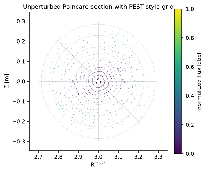
We trace field lines of the unperturbed equilibrium and record crossings at the \(\varphi=0\) plane. The result is the raw sampled geometry: useful, but not yet a topological object. Later cells add the promotion layer by overlaying resonant surfaces, X/O markers, local stable branches, and a PEST-style coordinate grid.
Crossings are cached to pyna_output/poincare_unperturbed.json.
[3]:
CACHE_UNPERT = pathlib.Path('pyna_output/poincare_unperturbed.json')
CACHE_UNPERT.parent.mkdir(exist_ok=True)

if CACHE_UNPERT.exists():
    _d = json.loads(CACHE_UNPERT.read_text())
    R_cross_u = np.array(_d['R'])
    Z_cross_u = np.array(_d['Z'])
    print(f'Loaded from cache: {len(R_cross_u)} crossings')
else:
    n_fieldlines = 15
    n_turns = 50
    dt = 0.08
    t_max = n_turns * 2 * np.pi * eq.R0

    R_starts = np.linspace(eq.R0 + 0.04*eq.r0, eq.R0 + 0.92*eq.r0, n_fieldlines)
    start_pts = np.zeros((n_fieldlines, 3))
    start_pts[:, 0] = R_starts
    start_pts[:, 2] = 0.0

    sections_u = [ToroidalSection(phi0=0.0)]
    print(f'Tracing {n_fieldlines} field lines x {n_turns} turns (dt={dt}, t_max={t_max:.1f} m)...')

    pmap_u = poincare_from_fieldlines(
        eq.field_func,
        start_pts,
        sections_u,
        t_max=t_max,
        dt=dt,
    )
    arr_u = pmap_u.crossing_array(0)
    R_cross_u = arr_u[:, 0]
    Z_cross_u = arr_u[:, 1]
    print(f'Computed: {len(R_cross_u)} crossings. Caching...')
    CACHE_UNPERT.write_text(json.dumps({'R': R_cross_u.tolist(), 'Z': Z_cross_u.tolist()}))
    print('Cached.')

fig_u, ax_u = plt.subplots(figsize=(4.7, 4.3), constrained_layout=True)
draw_pest_grid(ax_u, eq, alpha=0.22)
psi_pts = np.clip(((R_cross_u - eq.R0)**2 + Z_cross_u**2) / eq.r0**2, 0, 1)
draw_poincare_points(
    ax_u,
    R_cross_u,
    Z_cross_u,
    values=psi_pts,
    cmap='viridis',
    point_size=1.8,
    alpha=0.50,
    rasterized=False,
)
sm_u = plt.cm.ScalarMappable(cmap='viridis', norm=Normalize(0, 1))
fig_u.colorbar(sm_u, ax=ax_u, label='normalized flux label', shrink=0.82)
lim = 1.15 * eq.r0
ax_u.set_xlim(eq.R0 - lim, eq.R0 + lim)
ax_u.set_ylim(-lim, lim)
ax_u.set_aspect('equal')
ax_u.set_xlabel('R [m]')
ax_u.set_ylabel('Z [m]')
ax_u.set_title('Unperturbed Poincare section with PEST-style grid')
plt.show()
Loaded from cache: 735 crossings
[RMP_FIELD] Define and visualise the RMP perturbation field#
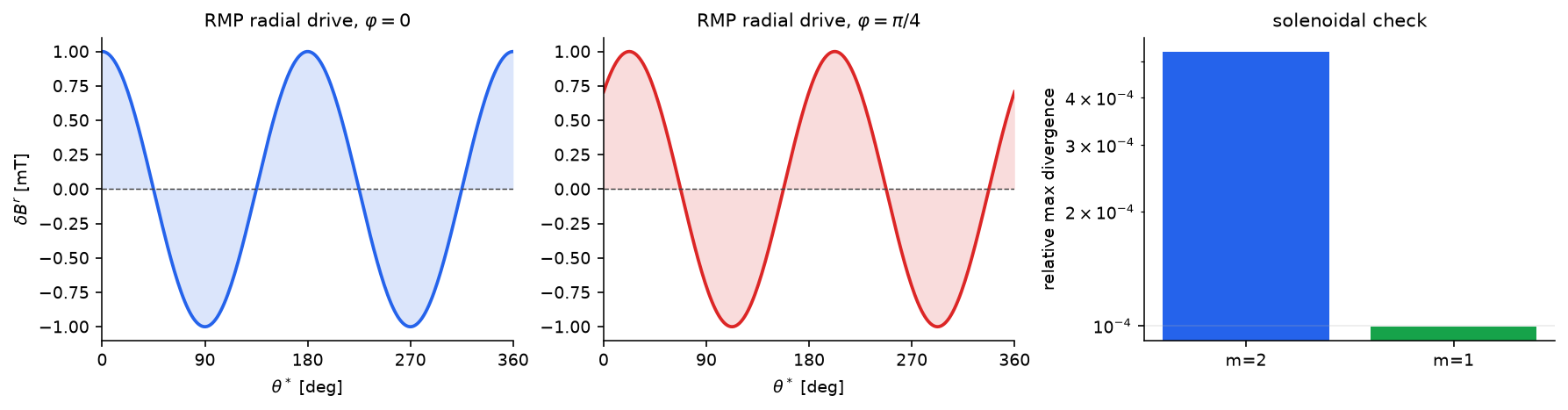
We apply a single-mode RMP with base mode \((m,n)=(2,1)\) and amplitude \(\delta B=1\) mT. The user-facing template is
but radial_rmp_field_template also adds the compensating poloidal/toroidal components needed to make the full cylindrical vector field divergence-free in the local circular-shell metric. The plotted radial projection is still the familiar resonant drive \(\delta B^r\).
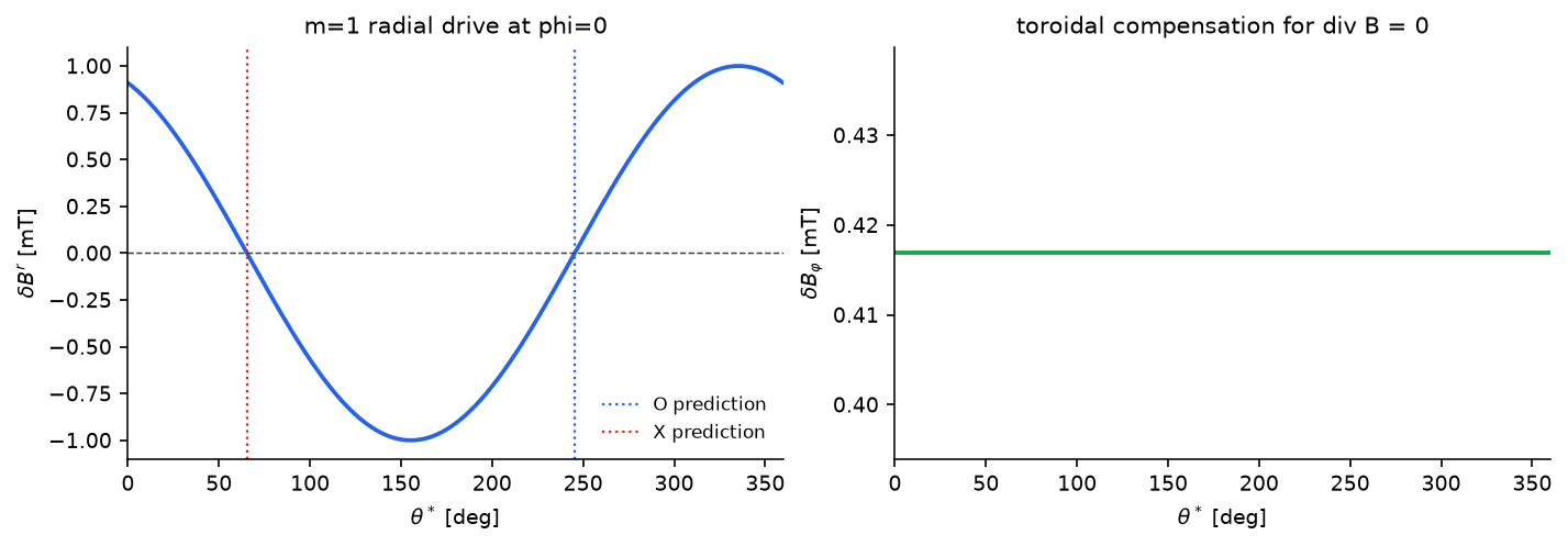
The same helper supports the important m=1 branch; that case needs a toroidal component because the radial divergence contains a theta-independent part.
[4]:
base_m, base_n = 2, 1
B_rmp = 1e-3  # 1 mT

delta_B_RMP = radial_rmp_field_template(
    base_m,
    base_n,
    amplitude=B_rmp,
    phase=0.0,
    axis_R=eq.R0,
)

psi_res_21 = eq.resonant_psi(2, 1)[0]
r_res_21 = np.sqrt(psi_res_21) * eq.r0
print(f'q=2/1 resonant surface: psi={psi_res_21:.3f}, r={r_res_21*100:.1f} cm')
print(f'delta_B/B0 = {B_rmp/eq.B0*100:.3f}%')

r_check = np.linspace(0.08, 0.28, 7)
div_m2 = circular_shell_divergence_diagnostic(
    delta_B_RMP,
    axis_R=eq.R0,
    r_values=r_check,
    n_theta=192,
    n_phi=192,
)
delta_B_m1_demo = radial_rmp_field_template(
    1,
    1,
    amplitude=B_rmp,
    phase=0.35,
    axis_R=eq.R0,
)
div_m1 = circular_shell_divergence_diagnostic(
    delta_B_m1_demo,
    axis_R=eq.R0,
    r_values=r_check,
    n_theta=192,
    n_phi=192,
)

print('Divergence diagnostics for the full vector perturbation:')
print('{:<8} {:>12} {:>12} {:>12}'.format('mode', 'max |div|', 'rms |div|', 'rel max'))
for label, diag in [('m=2', div_m2), ('m=1', div_m1)]:
    print(f'{label:<8} {diag.max_abs:12.3e} {diag.rms:12.3e} {diag.relative_max:12.3e}')

theta_arr = np.linspace(0, 2*np.pi, 240)
R_res = eq.R0 + r_res_21 * np.cos(theta_arr)
Z_res = r_res_21 * np.sin(theta_arr)

fig_rmp, axes_rmp = plt.subplots(1, 3, figsize=(11.8, 3.0), constrained_layout=True)
for ax, phi_val, phi_label, color in [
    (axes_rmp[0], 0.0, r'$\varphi=0$', '#2563eb'),
    (axes_rmp[1], np.pi/4, r'$\varphi=\pi/4$', '#dc2626'),
]:
    BR, BZ, _ = delta_B_RMP(R_res, Z_res, phi_val)
    dBpsi = BR*np.cos(theta_arr) + BZ*np.sin(theta_arr)
    ax.plot(np.degrees(theta_arr), dBpsi * 1e3, color=color, linewidth=1.8)
    ax.fill_between(np.degrees(theta_arr), 0, dBpsi * 1e3, color=color, alpha=0.16, linewidth=0)
    ax.axhline(0, color='0.25', lw=0.7, linestyle='--')
    ax.set_xlabel(r'$\theta^*$ [deg]')
    ax.set_title(f'RMP radial drive, {phi_label}')
    ax.set_xlim(0, 360)
    ax.set_xticks([0, 90, 180, 270, 360])
axes_rmp[0].set_ylabel(r'$\delta B^r$ [mT]')

axes_rmp[2].bar(['m=2', 'm=1'], [div_m2.relative_max, div_m1.relative_max], color=['#2563eb', '#16a34a'])
axes_rmp[2].set_yscale('log')
axes_rmp[2].set_ylabel('relative max divergence')
axes_rmp[2].set_title('solenoidal check')
axes_rmp[2].grid(True, axis='y', alpha=0.25)
plt.show()
print('Divergence-free RMP field defined and visualised.')
q=2/1 resonant surface: psi=0.167, r=12.2 cm
delta_B/B0 = 0.040%
Divergence diagnostics for the full vector perturbation:
mode        max |div|    rms |div|      rel max
m=2         6.642e-06    3.148e-06    5.300e-04
m=1         1.804e-06    7.949e-07    9.946e-05
Divergence-free RMP field defined and visualised.
[M1_RMP] m=1 phase-control mini-case#
The m=1 perturbation is common enough that it should not be treated as an edge case. Here the same divergence-free template drives a (1,1) resonance in a simple q=1 equilibrium. We verify three things in one short calculation: the field is numerically solenoidal, the extracted b_{1,-1} phase follows the template phase, and the predicted O/X points land on the zero crossings of the radial drive.
[5]:
eq_m1 = simple_stellarator(
    R0=eq.R0,
    r0=eq.r0,
    B0=eq.B0,
    q0=0.75,
    q1=1.25,
    m_h=eq.m_h,
    n_h=eq.n_h,
    epsilon_h=0.0,
)
m1_phase = 0.43
delta_B_m1 = radial_rmp_field_template(
    1,
    1,
    amplitude=B_rmp,
    phase=m1_phase,
    axis_R=eq_m1.R0,
)
psi_res_m1 = eq_m1.resonant_psi(1, 1)[0]
r_res_m1 = np.sqrt(psi_res_m1) * eq_m1.r0
m1_diag = circular_shell_divergence_diagnostic(
    delta_B_m1,
    axis_R=eq_m1.R0,
    r_values=np.linspace(0.08, 0.28, 7),
    n_theta=192,
    n_phi=192,
)
component_m1 = find_resonant_components_analytic(
    eq_m1,
    delta_B_m1,
    base_m=1,
    base_n=1,
    max_harmonic=1,
    n_theta=128,
    n_phi=64,
    min_amplitude=1e-16,
)[0]

print(f'm=1 resonant surface: psi={psi_res_m1:.3f}, r={r_res_m1*100:.1f} cm')
print(f'arg b_(1,-1) = {np.angle(component_m1.b_mn):.6f} rad, template phase = {m1_phase:.6f} rad')
print(f'|b_(1,-1)| = {abs(component_m1.b_mn):.3e} T, expected about B_rmp/2 = {0.5*B_rmp:.3e} T')
print(f'm=1 divergence relative max = {m1_diag.relative_max:.3e}')
print(f'O-point theta = {np.degrees(component_m1.opoint_theta):.2f} deg')
print(f'X-point theta = {np.degrees(component_m1.xpoint_theta):.2f} deg')

theta_m1 = np.linspace(0, 2*np.pi, 361)
R_m1 = eq_m1.R0 + r_res_m1*np.cos(theta_m1)
Z_m1 = r_res_m1*np.sin(theta_m1)
BR_m1, BZ_m1, Bphi_m1 = delta_B_m1(R_m1, Z_m1, 0.0)
dBr_m1 = BR_m1*np.cos(theta_m1) + BZ_m1*np.sin(theta_m1)

fig_m1, (ax_m1, ax_m1b) = plt.subplots(1, 2, figsize=(9.4, 3.2), constrained_layout=True)
ax_m1.plot(np.degrees(theta_m1), dBr_m1*1e3, color='#2563eb', lw=1.8)
ax_m1.axhline(0, color='0.25', lw=0.7, ls='--')
ax_m1.axvline(np.degrees(component_m1.opoint_theta), color='#2563eb', lw=1.1, ls=':', label='O prediction')
ax_m1.axvline(np.degrees(component_m1.xpoint_theta), color='#dc2626', lw=1.1, ls=':', label='X prediction')
ax_m1.set_xlim(0, 360)
ax_m1.set_xlabel(r'$\theta^*$ [deg]')
ax_m1.set_ylabel(r'$\delta B^r$ [mT]')
ax_m1.set_title('m=1 radial drive at phi=0')
ax_m1.legend(frameon=False, fontsize=8)

ax_m1b.plot(np.degrees(theta_m1), Bphi_m1*1e3, color='#16a34a', lw=1.8)
ax_m1b.set_xlim(0, 360)
ax_m1b.set_xlabel(r'$\theta^*$ [deg]')
ax_m1b.set_ylabel(r'$\delta B_\varphi$ [mT]')
ax_m1b.set_title('toroidal compensation for div B = 0')
plt.show()
  k=1: (1,1) ψ_res=0.500 q_res=1.000 |b_mn|=5.000e-04 phase_arg=24.6° w_ψ=0.1265 (2.68 cm) θ_O=245.4° θ_X=65.4°
m=1 resonant surface: psi=0.500, r=21.2 cm
arg b_(1,-1) = 0.430000 rad, template phase = 0.430000 rad
|b_(1,-1)| = 5.000e-04 T, expected about B_rmp/2 = 5.000e-04 T
m=1 divergence relative max = 9.946e-05
O-point theta = 245.36 deg
X-point theta = 65.36 deg
[RESONANT_COMPONENTS] Find resonant Fourier components#
We decompose the RMP field on each resonant flux surface using a 2D FFT and extract the amplitudes of the resonant \((m_k, n_k) = k\times(2,1)\) harmonics. The island half-width is given by the Rutherford formula:
Results are cached to pyna_output/rmp_components.json.
[6]:
CACHE_COMP = pathlib.Path('pyna_output/rmp_components.json')
CACHE_COMP.parent.mkdir(exist_ok=True)

print('Computing resonant components (n_theta=32, n_phi=16)...')
components = find_resonant_components_analytic(
    eq, delta_B_RMP, base_m=base_m, base_n=base_n,
    max_harmonic=3, n_theta=32, n_phi=16,
)
print(f'Found {len(components)} resonant components.')

# Cache as JSON
_comp_data = [{
    'm': c.m, 'n': c.n, 'harmonic_order': c.harmonic_order,
    'b_mn_real': float(c.b_mn.real), 'b_mn_imag': float(c.b_mn.imag),
    'psi_res': float(c.psi_res), 'q_res': float(c.q_res),
    'half_width_psi': float(c.half_width_psi),
    'half_width_r': float(c.half_width_r),
    'opoint_theta': float(c.opoint_theta),
    'xpoint_theta': float(c.xpoint_theta),
    'q_prime_sign': int(c.q_prime_sign),
} for c in components]
CACHE_COMP.write_text(json.dumps(_comp_data, indent=2))
print('Cached to', CACHE_COMP)

# Print table
print()
print(f'{"k":>3}  {"(m,n)":>8}  {"psi_res":>8}  {"q_res":>6}  {"b_mn|":>10}  {"w_psi":>8}  {"w_r (cm)":>10}  {"theta_O":>8}  {"theta_X":>8}')
print('-'*80)
for c in components:
    print(f'{c.harmonic_order:>3}  ({c.m},{c.n}){"":>4}  {c.psi_res:>8.4f}  {c.q_res:>6.3f}  {abs(c.b_mn):>10.3e}  {c.half_width_psi:>8.4f}  {c.half_width_r*100:>10.2f}  {np.degrees(c.opoint_theta):>8.1f}  {np.degrees(c.xpoint_theta):>8.1f}')
Computing resonant components (n_theta=32, n_phi=16)...
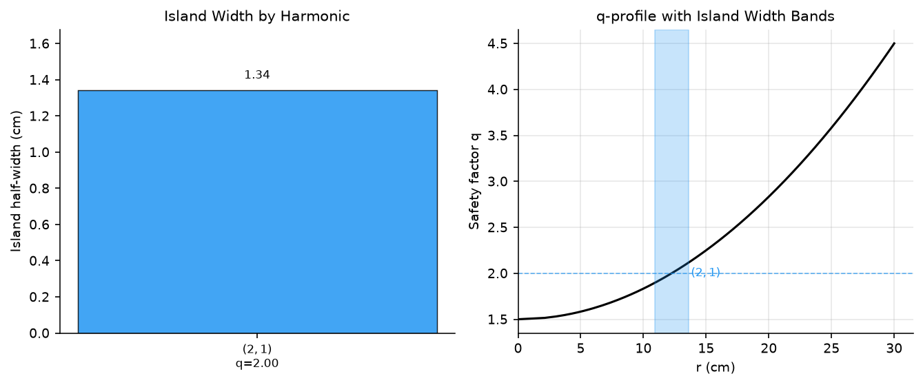
  k=1: (2,1) ψ_res=0.167 q_res=2.000 |b_mn|=5.000e-04 phase_arg=-0.0° w_ψ=0.0365 (1.34 cm) θ_O=135.0° θ_X=45.0°
  k=2: (4,2) — |b_mn|=4.57e-21 below threshold
  k=3: (6,3) — |b_mn|=1.98e-20 below threshold
Found 1 resonant components.
Cached to pyna_output/rmp_components.json

  k     (m,n)   psi_res   q_res       b_mn|     w_psi    w_r (cm)   theta_O   theta_X
--------------------------------------------------------------------------------
  1  (2,1)        0.1667   2.000   5.000e-04    0.0365        1.34     135.0      45.0
[POINCARE_PERTURBED] Geometry promotion: crossings -> X/O points -> manifolds#
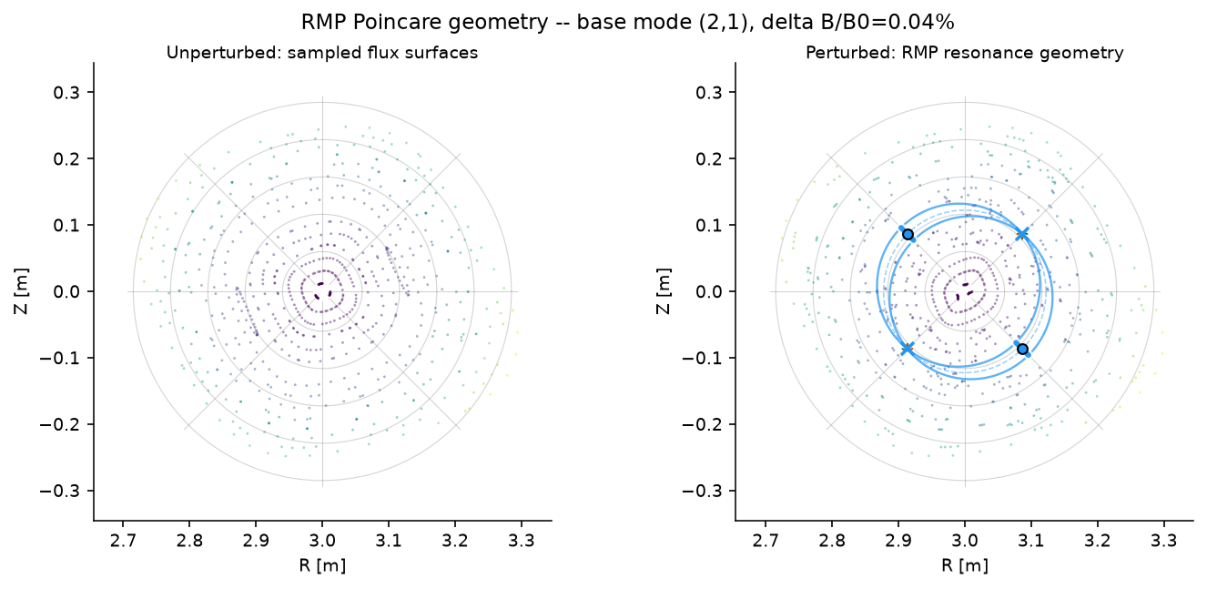
The perturbed trace gives sampled Poincare points. The analytic RMP spectrum gives fixed-point and island-width predictions. pyna.plot.draw_rmp_resonance_section combines them into one section geometry:
Poincare points colored by flux label;
PEST-style \((S,\theta^*)\) grid lines;
resonant surfaces for each harmonic;
O-points and X-points from the analytic fixed-point formula;
O-point radial bars whose length is set by the resonant Fourier amplitude;
local stable separatrix branches born from the X-points.
This is the same promotion idea used by the general geometry workflow: raw samples are kept distinct from persistent geometric objects and overlays until an explicit model or diagnostic justifies the promotion.
[7]:
# Perturbed field_func
# --------------------
def field_func_perturbed(rzphi_1d):
    """Unit-tangent dRZphi/ds for the field-line ODE with RMP added."""
    rzphi_1d = np.asarray(rzphi_1d, dtype=float)
    R, Z, phi = rzphi_1d[0], rzphi_1d[1], rzphi_1d[2]
    theta = np.arctan2(Z, R - R0_eq)
    psi = eq.psi_ax(R, Z)
    q = float(eq.q_of_psi(psi))
    r_minor = np.sqrt((R - R0_eq)**2 + Z**2)
    B_phi = eq.B0 * eq.R0 / R
    B_pol = B_phi * r_minor / (R * max(abs(q), 1e-3))
    if r_minor > 1e-10:
        BR0 = -B_pol * np.sin(theta)
        BZ0 =  B_pol * np.cos(theta)
    else:
        BR0 = BZ0 = 0.0
    delta_BR_eq = eq.epsilon_h * eq.B0 * psi * np.cos(eq.m_h * theta - eq.n_h * phi)
    db = delta_B_RMP(R, Z, phi)
    BR_tot = BR0 + delta_BR_eq + db[0]
    BZ_tot = BZ0 + db[1]
    B_phi_tot = B_phi + db[2]
    B_mag = np.sqrt(BR_tot**2 + BZ_tot**2 + B_phi_tot**2) + 1e-30
    return np.array([BR_tot/B_mag, BZ_tot/B_mag, B_phi_tot/(R*B_mag)])

CACHE_PERT = pathlib.Path('pyna_output/poincare_perturbed_divfree.json')
CACHE_PERT.parent.mkdir(exist_ok=True)

phi_sections_deg = [0, 60, 120, 180, 240, 300]
phi_sections = np.array(phi_sections_deg) * np.pi / 180.0

if CACHE_PERT.exists():
    _d = json.loads(CACHE_PERT.read_text())
    all_sections_data = _d['sections']
    print(f'Loaded perturbed Poincare from cache ({len(all_sections_data)} sections).')
else:
    sections_p = [ToroidalSection(phi0=ph) for ph in phi_sections]
    n_fieldlines, n_turns, dt = 15, 50, 0.08
    t_max = n_turns * 2 * np.pi * eq.R0
    start_pts = np.zeros((n_fieldlines, 3))
    start_pts[:, 0] = np.linspace(eq.R0 + 0.04*eq.r0, eq.R0 + 0.92*eq.r0, n_fieldlines)

    print(f'Tracing {n_fieldlines} field lines x {n_turns} turns (t_max={t_max:.1f} m)...')
    pmap_p = poincare_from_fieldlines(field_func_perturbed, start_pts, sections_p, t_max=t_max, dt=dt)
    all_sections_data = []
    for i_sec, phi_deg in enumerate(phi_sections_deg):
        arr = pmap_p.crossing_array(i_sec)
        print(f'  phi={phi_deg} deg: {len(arr)} crossings')
        all_sections_data.append({'R': arr[:, 0].tolist() if len(arr) else [], 'Z': arr[:, 1].tolist() if len(arr) else []})
    CACHE_PERT.write_text(json.dumps({'phi_sections_deg': phi_sections_deg, 'sections': all_sections_data}))
    print('Computed and cached.')

R_cross_p0 = np.array(all_sections_data[0]['R'])
Z_cross_p0 = np.array(all_sections_data[0]['Z'])
print(f'phi=0 section: {len(R_cross_p0)} crossings')

fig2, (axL, axR) = plt.subplots(1, 2, figsize=(9.4, 4.2), constrained_layout=True)

# The low-level plot layers are independently selectable by name.
draw_rmp_resonance_section(
    axL,
    R_cross_u,
    Z_cross_u,
    eq=eq,
    components=[],
    phi=0.0,
    title='Unperturbed: sampled flux surfaces',
    overlays=('pest_grid', 'poincare'),
    point_size=1.8,
    point_alpha=0.46,
)
draw_rmp_resonance_section(
    axR,
    R_cross_p0,
    Z_cross_p0,
    eq=eq,
    components=components,
    phi=0.0,
    colors=ISLAND_CMAPS,
    title='Perturbed: RMP resonance geometry',
    overlays=('pest_grid', 'poincare', 'resonant_surfaces', 'stable_branches', 'island_width_bars', 'xo'),
    point_size=1.8,
    point_alpha=0.46,
)

fig2.suptitle(
    f'RMP Poincare geometry -- base mode ({base_m},{base_n}), '
    f'delta B/B0={B_rmp/eq.B0*100:.2f}%',
    fontsize=11,
)
plt.show()
Loaded perturbed Poincare from cache (6 sections).
phi=0 section: 735 crossings
[CYNA_FIXED_POINTS] Newton fixed points versus RMP spectrum phases#
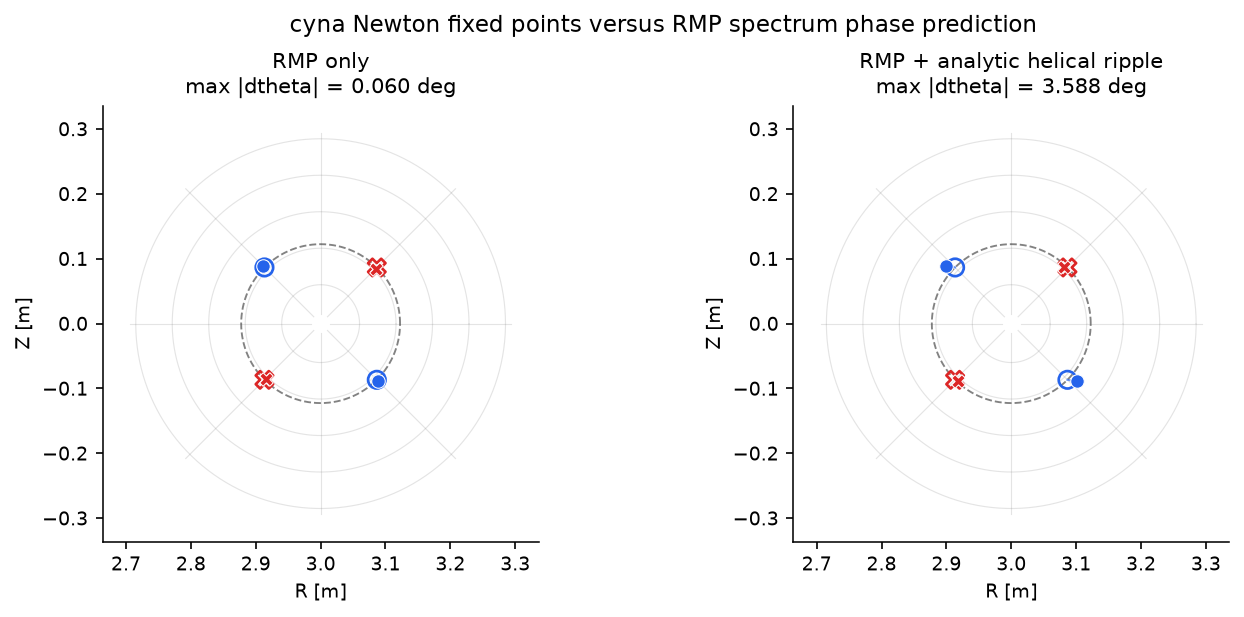
The RMP spectrum predicts first-order O/X-point phases. Here we use the accelerated cyna Newton map to refine those seeds into true periodic-orbit fixed points, then measure the phase error. The RMP-only case is a code sanity check; adding the analytic helical ripple shows the finite-amplitude/model shift that the first-order spectrum intentionally ignores.
[8]:
# Build a physical cylindrical field for cyna and compare Newton fixed points.
def row_newton_theta_deg(row, eq_case):
    axis_R, axis_Z = eq_case.magnetic_axis
    theta = np.arctan2(row.newton_Z - axis_Z, row.newton_R - axis_R) % (2*np.pi)
    return float(np.degrees(theta))


cyna_rows_by_case = {}
cyna_eq_by_case = {}
if components:
    eq_rmp_only = simple_stellarator(
        R0=eq.R0, r0=eq.r0, B0=eq.B0,
        q0=eq.q0, q1=eq.q1,
        m_h=eq.m_h, n_h=eq.n_h, epsilon_h=0.0,
    )
    try:
        for case_label, eq_case in [
            ('RMP only', eq_rmp_only),
            ('RMP + analytic helical ripple', eq),
        ]:
            print(f'Building cyna field: {case_label}')
            field_case = sample_stellarator_cylindrical_field(
                eq_case,
                delta_B_RMP,
                nR=128,
                nPhi=128,
                label=f'analytic_rmp_for_cyna_{case_label.replace(" ", "_").lower()}',
            )
            rows = compare_cyna_fixed_points_for_component(
                field_case,
                components[0],
                eq_case,
                DPhi=0.015,
                max_iter=80,
                tol=1e-11,
                n_threads=4,
            )
            cyna_rows_by_case[case_label] = rows
            cyna_eq_by_case[case_label] = eq_case
    except ImportError as exc:
        print('cyna fixed-point comparison skipped:', exc)

if cyna_rows_by_case:
    print()
    header = '{:<30} {:>4} {:>6} {:>9} {:>9} {:>10} {:>11} {:>11} {:>11}'.format(
        'case', 'kind', 'branch', 'theta*', 'theta_N', 'dtheta', 'm*dtheta', 'dr [cm]', 'residual'
    )
    print(header)
    print('-' * len(header))
    for case_label, rows in cyna_rows_by_case.items():
        eq_case = cyna_eq_by_case[case_label]
        for row in rows:
            theta_n = row_newton_theta_deg(row, eq_case)
            print('{:<30} {:>4} {:>6d} {:>9.3f} {:>9.3f} {:>10.4f} {:>11.4f} {:>11.4f} {:>11.1e}'.format(
                case_label,
                row.predicted_kind + '/' + (row.newton_kind or '?'),
                row.branch,
                row.predicted_theta_deg,
                theta_n,
                row.theta_error_deg,
                row.helical_phase_error_deg,
                row.radial_error_cm,
                row.residual,
            ))
        max_dtheta = max(abs(row.theta_error_deg) for row in rows)
        max_helical = max(abs(row.helical_phase_error_deg) for row in rows)
        print(f'  -> {case_label}: max |dtheta|={max_dtheta:.4f} deg, max |m*dtheta|={max_helical:.4f} deg')

if cyna_rows_by_case:
    fig_cmp, axes_cmp = plt.subplots(1, len(cyna_rows_by_case), figsize=(9.2, 4.0), constrained_layout=True)
    axes_cmp = np.atleast_1d(axes_cmp)
    for ax, (case_label, rows) in zip(axes_cmp, cyna_rows_by_case.items()):
        eq_case = cyna_eq_by_case[case_label]
        draw_pest_grid(ax, eq_case, alpha=0.18)
        r_res = np.sqrt(components[0].psi_res) * eq_case.r0
        theta_ring = np.linspace(0, 2*np.pi, 361)
        ax.plot(eq_case.R0 + r_res*np.cos(theta_ring), r_res*np.sin(theta_ring),
                color='0.25', lw=0.9, ls='--', alpha=0.65)
        for row in rows:
            color = '#2563eb' if row.predicted_kind == 'O' else '#dc2626'
            marker = 'o' if row.predicted_kind == 'O' else 'X'
            ax.plot([row.predicted_R, row.newton_R], [row.predicted_Z, row.newton_Z],
                    color=color, lw=1.0, alpha=0.65)
            ax.scatter(row.predicted_R, row.predicted_Z, marker=marker, s=70,
                       facecolors='none', edgecolors=color, linewidths=1.3, zorder=5)
            ax.scatter(row.newton_R, row.newton_Z, marker=marker, s=42,
                       color=color, edgecolors='white', linewidths=0.5, zorder=6)
        lim = 1.12 * eq_case.r0
        ax.set_xlim(eq_case.R0 - lim, eq_case.R0 + lim)
        ax.set_ylim(-lim, lim)
        ax.set_aspect('equal')
        ax.set_xlabel('R [m]')
        ax.set_ylabel('Z [m]')
        max_dtheta = max(abs(row.theta_error_deg) for row in rows)
        ax.set_title(f'{case_label}\nmax |dtheta| = {max_dtheta:.3f} deg')
    fig_cmp.suptitle('cyna Newton fixed points versus RMP spectrum phase prediction', fontsize=11)
    plt.show()
Building cyna field: RMP only
Building cyna field: RMP + analytic helical ripple

case                           kind branch    theta*   theta_N     dtheta    m*dtheta     dr [cm]    residual
-------------------------------------------------------------------------------------------------------------
RMP only                        O/O      0   315.000   314.940    -0.0602     -0.1203      0.2298     1.4e-14
RMP only                        O/O      1   135.000   135.059     0.0588      0.1176      0.2303     9.2e-15
RMP only                        X/X      0    45.000    44.940    -0.0600     -0.1200     -0.2520     4.7e-14
RMP only                        X/X      1   225.000   225.059     0.0588      0.1176     -0.2515     1.7e-14
  -> RMP only: max |dtheta|=0.0602 deg, max |m*dtheta|=0.1203 deg
RMP + analytic helical ripple   O/O      0   315.000   318.588     3.5877      7.1754      1.2050     5.0e-12
RMP + analytic helical ripple   O/O      1   135.000   138.420     3.4195      6.8391      1.1869     2.2e-15
RMP + analytic helical ripple   X/X      0    45.000    47.043     2.0428      4.0857     -0.2143     2.7e-12
RMP + analytic helical ripple   X/X      1   225.000   226.940     1.9400      3.8801     -0.2445     2.3e-12
  -> RMP + analytic helical ripple: max |dtheta|=3.5877 deg, max |m*dtheta|=7.1754 deg
[NONRESONANT_DEFORMATION] Non-resonant ripple as flux-surface deformation#
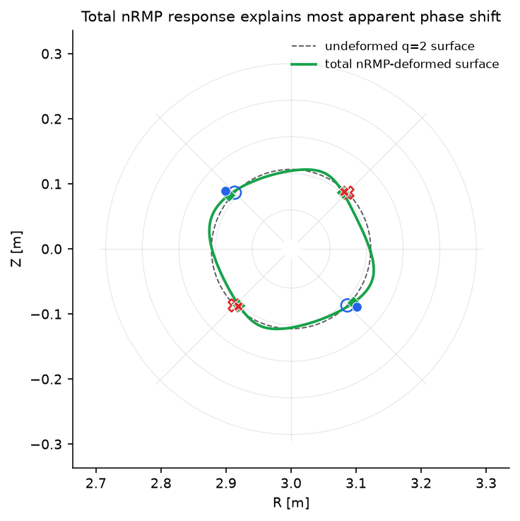
The helical ripple in this analytic equilibrium is not the resonant RMP component that opens the (m,n)=(2,1) island. It still changes the geometry of the nearby flux surface. If we compare Newton fixed points against the undeformed circular surface, that smooth displacement appears as an artificial phase error.
Here we sample the helical-ripple contribution to the field-line ODE,
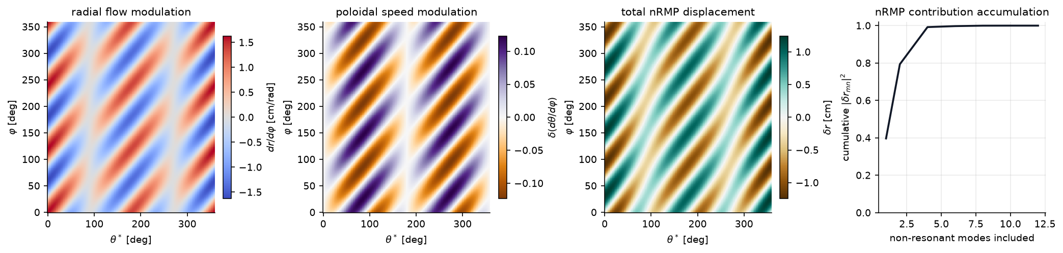
Fourier transform F_r and F_theta, and solve the non-resonant homological equation for every non-resonant coefficient. The response object keeps the total deformation and a contribution ranking; the ranking is a diagnostic, while the deformation used below is the full summed nRMP response.
[9]:
def helical_ripple_delta_B(eq_case):
    """Return the analytic helical-ripple contribution used by simple_stellarator."""
    def delta_B_helical(R, Z, phi):
        R_arr = np.asarray(R, dtype=float)
        Z_arr = np.asarray(Z, dtype=float)
        phi_arr = np.asarray(phi, dtype=float)
        theta = np.arctan2(Z_arr, R_arr - eq_case.R0)
        psi = eq_case.psi_ax(R_arr, Z_arr)
        dBR = eq_case.epsilon_h * eq_case.B0 * psi * np.cos(eq_case.m_h * theta - eq_case.n_h * phi_arr)
        return np.array([
            dBR,
            np.zeros_like(dBR, dtype=float),
            np.zeros_like(dBR, dtype=float),
        ])
    return delta_B_helical


def helical_velocity_response(eq_case, psi_res, n_theta=256, n_phi=256, include_shear=False):
    velocity = fieldline_velocity_spectrum_on_circular_surface(
        eq_case,
        helical_ripple_delta_B(eq_case),
        psi_res,
        n_theta=n_theta,
        n_phi=n_phi,
        m_max=8,
        n_max=8,
        min_amplitude=1e-12,
    )
    return velocity.nonresonant_response(include_shear=include_shear)


def helical_velocity_deformation(eq_case, psi_res, n_theta=256, n_phi=256, include_shear=False):
    response = helical_velocity_response(
        eq_case,
        psi_res,
        n_theta=n_theta,
        n_phi=n_phi,
        include_shear=include_shear,
    )
    return response.deformation, response.velocity.r_minor, response.velocity


case_label = 'RMP + analytic helical ripple'
if components and case_label in cyna_rows_by_case:
    rows = cyna_rows_by_case[case_label]
    eq_case = cyna_eq_by_case[case_label]
    response_helical = helical_velocity_response(eq_case, components[0].psi_res)
    deformation = response_helical.deformation
    velocity_helical = response_helical.velocity
    r_res = velocity_helical.r_minor
    projected_rows = project_fixed_points_to_deformed_surface(
        rows,
        eq_case,
        deformation,
        r_minor=r_res,
        theta_window=0.35,
    )

    print(
        'nRMP total response uses '
        f'{response_helical.n_nonresonant_modes} non-resonant modes '
        f'and excludes {response_helical.n_resonant_modes} resonant modes.'
    )
    print('Largest nRMP response contributors; these rank the sum but do not replace it:')
    print('{:>8} {:>12} {:>14} {:>14}'.format('(m,n)', 'detuning', '|delta_r_mn| cm', 'cum frac'))
    for contrib in response_helical.contribution_rows(top=6):
        print('({:>2d},{:>2d}) {:>12.3e} {:>14.4f} {:>14.3f}'.format(
            contrib.m,
            contrib.n,
            contrib.detuning,
            100.0 * contrib.radial_response_weight,
            contrib.cumulative_fraction,
        ))
    print()

    raw_max = max(abs(row.theta_error_deg) for row in rows)
    corrected_max = max(abs(row.theta_error_deg) for row in projected_rows)
    nearest_max = max(row.distance_cm for row in projected_rows)
    print(f'Raw circular-surface max |dtheta|:       {raw_max:.4f} deg')
    print(f'Deformed-surface-coordinate max |dtheta|: {corrected_max:.4f} deg')
    print(f'Max Newton-to-deformed-section distance:  {nearest_max:.3f} cm')
    print()
    header = '{:<4} {:>6} {:>12} {:>16} {:>13}'.format(
        'kind', 'branch', 'raw dtheta', 'deformed dtheta', 'distance [cm]'
    )
    print(header)
    print('-' * len(header))
    for row, proj in zip(rows, projected_rows):
        print('{:<4} {:>6d} {:>12.4f} {:>16.4f} {:>13.3f}'.format(
            row.predicted_kind,
            row.branch,
            row.theta_error_deg,
            proj.theta_error_deg,
            proj.distance_cm,
        ))

    theta_line = np.linspace(0.0, 2*np.pi, 721)
    R_circ = eq_case.R0 + r_res*np.cos(theta_line)
    Z_circ = r_res*np.sin(theta_line)
    R_def, Z_def = deformed_circular_section_rz(eq_case, r_res, deformation, theta_line)

    fig_def, ax_def = plt.subplots(figsize=(5.2, 4.8), constrained_layout=True)
    draw_pest_grid(ax_def, eq_case, alpha=0.16)
    ax_def.plot(R_circ, Z_circ, color='0.35', lw=0.9, ls='--', label='undeformed q=2 surface')
    ax_def.plot(R_def, Z_def, color='#16a34a', lw=1.8, label='total nRMP-deformed surface')

    for row, proj in zip(rows, projected_rows):
        color = '#2563eb' if row.predicted_kind == 'O' else '#dc2626'
        marker = 'o' if row.predicted_kind == 'O' else 'X'
        ax_def.plot([row.predicted_R, row.newton_R], [row.predicted_Z, row.newton_Z],
                    color=color, lw=0.8, alpha=0.35)
        ax_def.plot([proj.closest_R, row.newton_R], [proj.closest_Z, row.newton_Z],
                    color=color, lw=1.1, ls=':', alpha=0.9)
        ax_def.scatter(row.predicted_R, row.predicted_Z, marker=marker, s=72,
                       facecolors='none', edgecolors=color, linewidths=1.2, zorder=5)
        ax_def.scatter(proj.closest_R, proj.closest_Z, marker='D', s=42,
                       color='#16a34a', edgecolors='white', linewidths=0.45, zorder=6)
        ax_def.scatter(row.newton_R, row.newton_Z, marker=marker, s=44,
                       color=color, edgecolors='white', linewidths=0.5, zorder=7)

    lim = 1.12 * eq_case.r0
    ax_def.set_xlim(eq_case.R0 - lim, eq_case.R0 + lim)
    ax_def.set_ylim(-lim, lim)
    ax_def.set_aspect('equal')
    ax_def.set_xlabel('R [m]')
    ax_def.set_ylabel('Z [m]')
    ax_def.set_title('Total nRMP response explains most apparent phase shift')
    ax_def.legend(frameon=False, loc='upper right', fontsize=8)
    plt.show()

    TT_h, PP_h, dr_h, dtheta_h = response_helical.real_fields()
    counts_h, cumulative_h = response_helical.cumulative_contribution()
    theta_deg_h = np.degrees(velocity_helical.theta)
    phi_deg_h = np.degrees(velocity_helical.phi)
    fig_flow, axes_flow = plt.subplots(1, 4, figsize=(13.8, 3.2), constrained_layout=True)
    panels = [
        (velocity_helical.radial_velocity * 100.0, r'$dr/d\varphi$ [cm/rad]', 'radial flow modulation', 'coolwarm'),
        (velocity_helical.poloidal_velocity, r'$\delta(d\theta/d\varphi)$', 'poloidal speed modulation', 'PuOr'),
        (dr_h * 100.0, r'$\delta r$ [cm]', 'total nRMP displacement', 'BrBG'),
    ]
    for ax, (data, cbar_label, title, cmap) in zip(axes_flow[:3], panels):
        vmax = np.nanmax(np.abs(data))
        im = ax.pcolormesh(
            theta_deg_h,
            phi_deg_h,
            data,
            shading='auto',
            cmap=cmap,
            vmin=-vmax,
            vmax=vmax,
        )
        ax.set_xlabel(r'$\theta^*$ [deg]')
        ax.set_ylabel(r'$\varphi$ [deg]')
        ax.set_title(title)
        fig_flow.colorbar(im, ax=ax, label=cbar_label, shrink=0.85)
    axes_flow[3].plot(counts_h, cumulative_h, color='#111827', lw=1.8)
    axes_flow[3].set_ylim(0, 1.02)
    axes_flow[3].set_xlabel('non-resonant modes included')
    axes_flow[3].set_ylabel(r'cumulative $|\delta r_{mn}|^2$')
    axes_flow[3].set_title('nRMP contribution accumulation')
    axes_flow[3].grid(True, alpha=0.25)
    plt.show()
else:
    print('Non-resonant deformation check skipped because cyna rows are unavailable.')
nRMP total response uses 12 non-resonant modes and excludes 2 resonant modes.
Largest nRMP response contributors; these rank the sum but do not replace it:
   (m,n)     detuning |delta_r_mn| cm       cum frac
(-4, 3)    1.000e+00         0.3755          0.397
( 4,-3)   -1.000e+00         0.3755          0.794
(-2, 3)    2.000e+00         0.1877          0.893
( 2,-3)   -2.000e+00         0.1877          0.992
(-5, 3)    5.000e-01         0.0306          0.995
( 5,-3)   -5.000e-01         0.0306          0.997

Raw circular-surface max |dtheta|:       3.5877 deg
Deformed-surface-coordinate max |dtheta|: 1.4748 deg
Max Newton-to-deformed-section distance:  0.822 cm

kind branch   raw dtheta  deformed dtheta distance [cm]
-------------------------------------------------------
O         0       3.5877           0.6159         0.822
O         1       3.4195           0.7933         0.783
X         0       2.0428          -1.4748         0.250
X         1       1.9400          -1.1567         0.196
[MIXED_SPECTRUM] Mixed RMP/nRMP workflow on one surface#
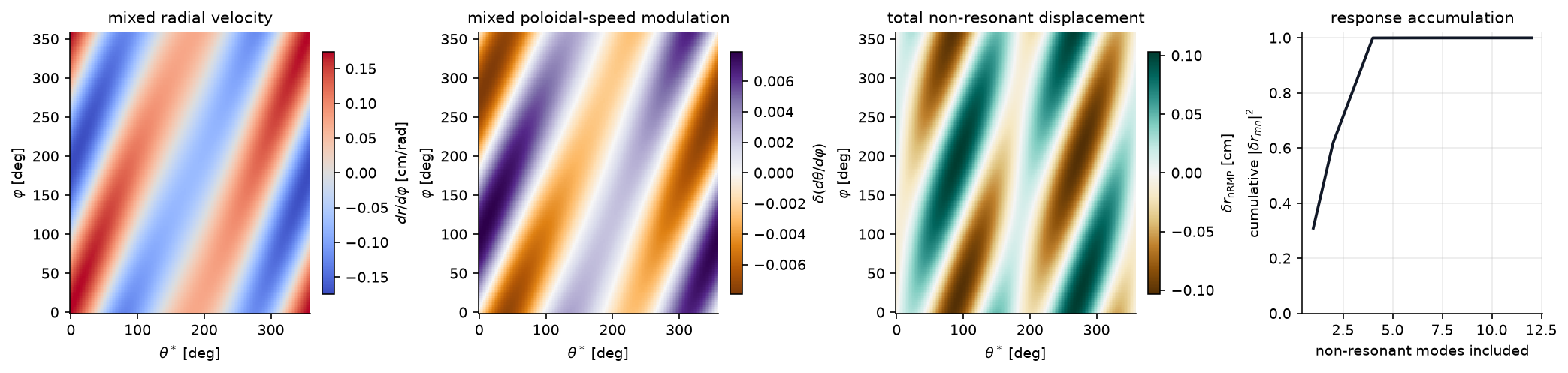
Real perturbations rarely contain one clean harmonic. This example superposes a resonant (2,1) RMP with two non-resonant components, including an m=1 term. The mode table classifies the sampled velocity spectrum, but it is only a diagnostic. The nRMP part of the calculation is the total response object, which sums every non-resonant row before drawing the smooth displacement and speed modulation.
[10]:
mixed_delta_B = compose_magnetic_perturbations(
    delta_B_RMP,
    radial_rmp_field_template(3, 1, amplitude=2.0e-4, phase=0.20, axis_R=eq.R0),
    radial_rmp_field_template(1, 1, amplitude=1.5e-4, phase=0.40, axis_R=eq.R0),
)

mixed_velocity = fieldline_velocity_spectrum_on_circular_surface(
    eq,
    mixed_delta_B,
    psi_res_21,
    n_theta=160,
    n_phi=128,
    m_max=5,
    n_max=4,
    min_amplitude=1e-13,
)
mixed_rows = rmp_nrmp_mode_rows(
    mixed_velocity.radial_spectrum,
    mixed_velocity.iota,
    resonance_tol=1e-10,
    top=12,
    min_amplitude=1e-8,
)
mixed_response = mixed_velocity.nonresonant_response(include_shear=True, resonance_tol=1e-10)

print(f'Local iota on q=2 surface: {mixed_velocity.iota:.6f}')
print(
    'Total nRMP response uses '
    f'{mixed_response.n_nonresonant_modes} non-resonant modes; '
    f'{mixed_response.n_resonant_modes} resonant modes are left for island analysis.'
)
print()
print('RMP/nRMP mode classification diagnostic:')
print('{:<5} {:>8} {:>12} {:>12} {:>12}'.format('kind', '(m,n)', 'detuning', '|F_r mn|', 'phase [deg]'))
print('-' * 56)
for row in mixed_rows:
    print('{:<5} ({:>2d},{:>2d}) {:>12.3e} {:>12.3e} {:>12.2f}'.format(
        row.kind,
        row.m,
        row.n,
        row.detuning,
        row.amplitude,
        row.phase_deg,
    ))

print()
print('Largest contributors to the total nRMP radial response:')
print('{:>8} {:>12} {:>14} {:>14}'.format('(m,n)', 'detuning', '|delta_r_mn| cm', 'cum frac'))
for contrib in mixed_response.contribution_rows(top=8):
    print('({:>2d},{:>2d}) {:>12.3e} {:>14.4f} {:>14.3f}'.format(
        contrib.m,
        contrib.n,
        contrib.detuning,
        100.0 * contrib.radial_response_weight,
        contrib.cumulative_fraction,
    ))

mixed_deformation = mixed_response.deformation
TT_mix, PP_mix, nonres_dr_mix, nonres_dtheta_mix = mixed_response.real_fields()
counts_mix, cumulative_mix = mixed_response.cumulative_contribution()

theta_deg_mix = np.degrees(mixed_velocity.theta)
phi_deg_mix = np.degrees(mixed_velocity.phi)
fig_mix, axes_mix = plt.subplots(1, 4, figsize=(13.8, 3.2), constrained_layout=True)
panels = [
    (mixed_velocity.radial_velocity * 100.0, r'$dr/d\varphi$ [cm/rad]', 'mixed radial velocity', 'coolwarm'),
    (mixed_velocity.poloidal_velocity, r'$\delta(d\theta/d\varphi)$', 'mixed poloidal-speed modulation', 'PuOr'),
    (nonres_dr_mix * 100.0, r'$\delta r_\mathrm{nRMP}$ [cm]', 'total non-resonant displacement', 'BrBG'),
]
for ax, (data, label, title, cmap) in zip(axes_mix[:3], panels):
    vmax = np.nanmax(np.abs(data))
    im = ax.pcolormesh(
        theta_deg_mix,
        phi_deg_mix,
        data,
        shading='auto',
        cmap=cmap,
        vmin=-vmax,
        vmax=vmax,
    )
    ax.set_xlabel(r'$\theta^*$ [deg]')
    ax.set_ylabel(r'$\varphi$ [deg]')
    ax.set_title(title)
    fig_mix.colorbar(im, ax=ax, label=label, shrink=0.86)
axes_mix[3].plot(counts_mix, cumulative_mix, color='#111827', lw=1.8)
axes_mix[3].set_ylim(0, 1.02)
axes_mix[3].set_xlabel('non-resonant modes included')
axes_mix[3].set_ylabel(r'cumulative $|\delta r_{mn}|^2$')
axes_mix[3].set_title('response accumulation')
axes_mix[3].grid(True, alpha=0.25)
plt.show()
Local iota on q=2 surface: 0.500000
Total nRMP response uses 12 non-resonant modes; 2 resonant modes are left for island analysis.

RMP/nRMP mode classification diagnostic:
kind     (m,n)     detuning     |F_r mn|  phase [deg]
--------------------------------------------------------
RMP   (-2, 1)    0.000e+00    6.087e-04        -0.23
RMP   ( 2,-1)    0.000e+00    6.087e-04         0.23
nRMP  (-3, 1)   -5.000e-01    1.442e-04        -9.53
nRMP  ( 3,-1)    5.000e-01    1.442e-04         9.53
nRMP  (-1, 1)    5.000e-01    1.131e-04       -18.07
nRMP  ( 1,-1)   -5.000e-01    1.131e-04        18.07
nRMP  ( 4,-1)    1.000e+00    5.144e-06        10.91
nRMP  (-4, 1)   -1.000e+00    5.144e-06       -10.91
nRMP  ( 0,-1)   -1.000e+00    3.906e-06        21.49
nRMP  ( 0, 1)    1.000e+00    3.906e-06       -21.49
nRMP  (-5, 1)   -1.500e+00    5.000e-08       -11.46
nRMP  ( 5,-1)    1.500e+00    5.000e-08        11.46

Largest contributors to the total nRMP radial response:
   (m,n)     detuning |delta_r_mn| cm       cum frac
(-3, 1)   -5.000e-01         0.0288          0.310
( 3,-1)    5.000e-01         0.0288          0.619
(-1, 1)    5.000e-01         0.0226          0.809
( 1,-1)   -5.000e-01         0.0226          1.000
( 4,-1)    1.000e+00         0.0005          1.000
(-4, 1)   -1.000e+00         0.0005          1.000
( 0, 1)    1.000e+00         0.0004          1.000
( 0,-1)   -1.000e+00         0.0004          1.000
[ORDER_ANALYSIS] Perturbation-order checks#
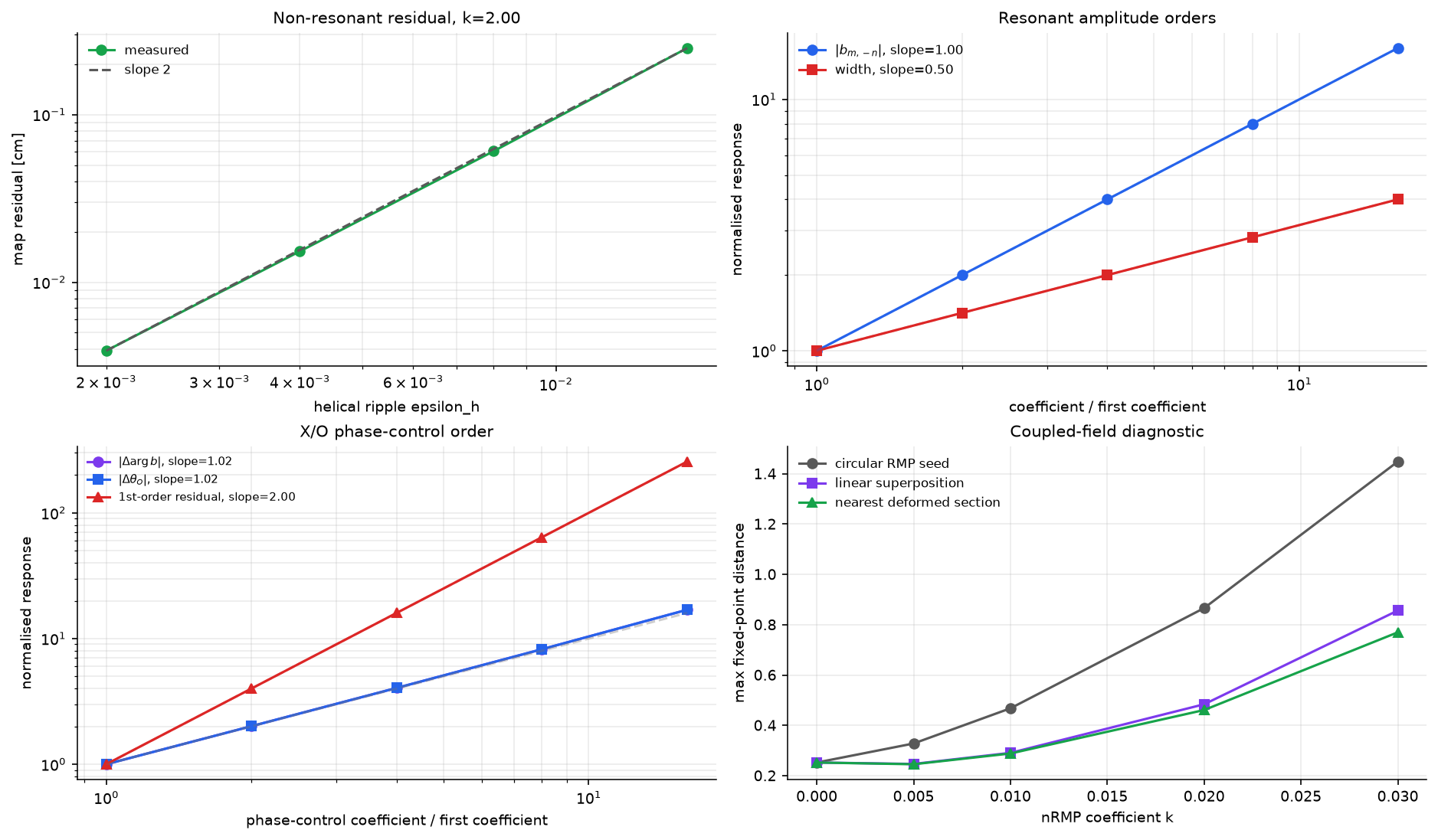
The reusable workflow now lives in a few small helpers: scan_nonresonant_residual_order, scan_rmp_amplitude_order, scan_rmp_phase_order, scan_rmp_resolution_convergence, and plot_perturbation_order_summary.
The expected orders are simple once the Fourier convention is fixed:
nRMP surface-shape residual: a first-order deformation should leave an
O(k^2)map residual.RMP resonant coefficient: for
delta B = k f, Fourier linearity gives|b_{m,-n}| ~ k.Island width: the Rutherford/Nardon pendulum width scales as
w ~ sqrt(|b_{m,-n}|), hencew ~ k^{1/2}.X/O phase: the phase is controlled by
arg(b_{m,-n}), not by amplitude. The exact relation ism*Delta theta_O + Delta arg(b_{m,-n}) = 0.
For phase-control order we use the divergence-free template radial_rmp_field_template. Its phase parameter changes the resonant coefficient phase while preserving div(delta B)=0, including the important m=1 case. We deliberately test a mildly nonlinear control phase alpha(k)=k+eta*k^2; the residual against the first-order raw-k law should therefore scale as O(k^2).
[11]:
def component_for_rmp_template(amplitude=1.0e-3, phase=0.0, n_theta=128, n_phi=64):
    return find_resonant_components_analytic(
        eq,
        radial_rmp_field_template(base_m, base_n, amplitude=amplitude, phase=phase, axis_R=eq.R0),
        base_m=base_m,
        base_n=base_n,
        max_harmonic=1,
        n_theta=n_theta,
        n_phi=n_phi,
        min_amplitude=1e-16,
        verbose=False,
    )[0]


def deformed_torus_map_residual(epsilon_h, n_alpha=12):
    eq_case = simple_stellarator(
        R0=eq.R0, r0=eq.r0, B0=eq.B0,
        q0=eq.q0, q1=eq.q1,
        m_h=eq.m_h, n_h=eq.n_h, epsilon_h=float(epsilon_h),
    )
    psi_res = eq_case.resonant_psi(base_m, base_n)[0]
    deformation, r_res, _ = helical_velocity_deformation(
        eq_case, psi_res, n_theta=128, n_phi=128, include_shear=True
    )
    iota = 1.0 / float(eq_case.q_of_psi(psi_res))

    def surface(alpha, phi):
        alpha_arr = np.asarray(alpha)
        return (
            r_res + deformation.section_r(alpha_arr, phi),
            alpha_arr + deformation.section_theta(alpha_arr, phi),
        )

    def rhs(phi, state):
        radius, theta = state
        R = eq_case.R0 + radius*np.cos(theta)
        psi_here = (radius / eq_case.r0)**2
        q_here = float(eq_case.q_of_psi(psi_here))
        Bphi = eq_case.B0 * eq_case.R0 / R
        delta_BR = eq_case.epsilon_h * eq_case.B0 * psi_here * np.cos(eq_case.m_h * theta - eq_case.n_h * phi)
        return [
            R * delta_BR * np.cos(theta) / Bphi,
            1.0/q_here - R * delta_BR * np.sin(theta) / (radius * Bphi),
        ]

    residual = deformed_surface_map_residual(
        surface,
        rhs,
        iota,
        alpha_values=np.linspace(0.0, 2*np.pi, n_alpha, endpoint=False),
        state_to_cartesian=lambda state, phi: [
            eq_case.R0 + float(state[0])*np.cos(float(state[1])),
            float(state[0])*np.sin(float(state[1])),
        ],
    )
    return residual.max_residual


def max_helical_deformation_cm(n_theta, n_phi):
    velocity = fieldline_velocity_spectrum_on_circular_surface(
        eq,
        helical_ripple_delta_B(eq),
        psi_res_21,
        n_theta=max(64, n_theta),
        n_phi=max(64, n_phi),
        m_max=8,
        n_max=8,
        min_amplitude=1e-12,
    )
    deformation = velocity.nonresonant_deformation(include_shear=True)
    TT, PP = np.meshgrid(velocity.theta, velocity.phi, indexing='xy')
    return 100.0 * float(np.nanmax(np.abs(deformation.real_field_r(TT, PP))))


nonres_eps = np.array([0.002, 0.004, 0.008, 0.016])
rmp_k = np.array([2.5e-4, 5e-4, 1e-3, 2e-3, 4e-3])
phase_controls = np.array([0.01, 0.02, 0.04, 0.08, 0.16])
phase_eta = 0.4

nonres_scan = scan_nonresonant_residual_order(nonres_eps, deformed_torus_map_residual)
rmp_amp_scan = scan_rmp_amplitude_order(
    rmp_k,
    lambda k: component_for_rmp_template(amplitude=k, phase=0.0, n_theta=64, n_phi=32),
)
phase_base = component_for_rmp_template(amplitude=1e-3, phase=0.0, n_theta=128, n_phi=64)
phase_scan = scan_rmp_phase_order(
    phase_controls,
    lambda k: component_for_rmp_template(
        amplitude=1e-3,
        phase=float(k) + phase_eta*float(k)*float(k),
        n_theta=128,
        n_phi=64,
    ),
    base_component=phase_base,
)
resolution_scan = scan_rmp_resolution_convergence(
    [(32, 16), (64, 32), (128, 64), (256, 128)],
    lambda n_theta, n_phi: component_for_rmp_template(
        amplitude=1e-3, phase=0.0, n_theta=n_theta, n_phi=n_phi
    ),
    deformation_metric_factory=max_helical_deformation_cm,
)

comp_pos = component_for_rmp_template(amplitude=1e-3, phase=0.0, n_theta=64, n_phi=32)
comp_neg = component_for_rmp_template(amplitude=-1e-3, phase=0.0, n_theta=64, n_phi=32)
sign_phase_jump_deg = float(np.degrees(np.angle(comp_neg.b_mn / comp_pos.b_mn)))

print(f'Non-resonant deformation residual slope = {nonres_scan.slope:.3f} (expected 2)')
print(f'Positive RMP: |b_mn| slope =             {rmp_amp_scan.b_fit.slope:.3f} (expected 1)')
print(f'Positive RMP: island half-width slope =  {rmp_amp_scan.width_fit.slope:.3f} (expected 0.5)')
print(f'Positive RMP: X/O phase span:           {rmp_amp_scan.phase_span_deg:.3e} deg')
print(f'Negative coefficient: arg jump:         {sign_phase_jump_deg:.1f} deg')
print(f'  +k: O={np.degrees(comp_pos.opoint_theta):.1f} deg, X={np.degrees(comp_pos.xpoint_theta):.1f} deg')
print(f'  -k: O={np.degrees(comp_neg.opoint_theta):.1f} deg, X={np.degrees(comp_neg.xpoint_theta):.1f} deg')
print(f'Phase template: |Delta arg b| slope =    {phase_scan.b_phase_fit.slope:.3f} (locally expected 1)')
print(f'Phase template: |Delta theta_O| vs |Delta arg b| slope = {phase_scan.opoint_vs_b_phase_fit.slope:.3f} (expected 1)')
print(f'Phase template: max |m Delta theta_O + Delta arg b|: {phase_scan.max_exact_relation_residual:.3e} rad')
print(f'Phase template: first-order residual slope = {phase_scan.first_order_residual_fit.slope:.3f} (expected 2)')

print()
print('Resolution convergence against the finest RMP spectrum grid:')
print('{:>8} {:>6} {:>12} {:>14} {:>14} {:>14}'.format(
    'n_theta', 'n_phi', 'rel |b| err', 'phase err deg', 'rel width err', 'max |dr| cm'
))
for row in resolution_scan.rows:
    print(f'{row.n_theta:8d} {row.n_phi:6d} {row.relative_b_error:12.3e} '
          f'{row.phase_error_deg:14.3e} {row.relative_width_error:14.3e} '
          f'{row.deformation_metric:14.4f}')

coupling_sweep = None
if components:
    component = components[0]

    def coupled_distances(eps_h):
        eq_case = simple_stellarator(
            R0=eq.R0, r0=eq.r0, B0=eq.B0,
            q0=eq.q0, q1=eq.q1,
            m_h=eq.m_h, n_h=eq.n_h, epsilon_h=float(eps_h),
        )
        rows = compare_cyna_fixed_points_for_component(
            sample_stellarator_cylindrical_field(
                eq_case, delta_B_RMP, nR=128, nPhi=128, label=f'coupled_rmp_eps_{eps_h:.3f}',
            ),
            component,
            eq_case,
            DPhi=0.015,
            max_iter=80,
            tol=1e-11,
            n_threads=4,
        )
        raw_cm = max(np.hypot(row.newton_R - row.predicted_R, row.newton_Z - row.predicted_Z) for row in rows) * 100.0
        if eps_h == 0.0:
            return raw_cm, raw_cm, raw_cm
        deformation, r_res, _ = helical_velocity_deformation(eq_case, component.psi_res, include_shear=True)
        superposed_cm = max(
            np.hypot(
                float(deformed_circular_section_rz(eq_case, r_res, deformation, row.predicted_theta)[0]) - row.newton_R,
                float(deformed_circular_section_rz(eq_case, r_res, deformation, row.predicted_theta)[1]) - row.newton_Z,
            ) for row in rows
        ) * 100.0
        projected = project_fixed_points_to_deformed_surface(rows, eq_case, deformation, r_minor=r_res)
        return raw_cm, superposed_cm, max(row.distance_cm for row in projected)

    try:
        coupling_sweep = scan_coupled_fixed_point_sweep(np.array([0.0, 0.005, 0.01, 0.02, 0.03]), coupled_distances)
    except ImportError as exc:
        print('Coupled cyna sweep skipped:', exc)

if coupling_sweep is not None:
    print()
    print('Coupled RMP + helical ripple, fixed RMP amplitude:')
    print('{:>9} {:>12} {:>16} {:>16}'.format('epsilon_h', 'raw [cm]', 'superposed [cm]', 'nearest [cm]'))
    for eps_h, raw_cm, superposed_cm, nearest_cm in zip(
        coupling_sweep.k, coupling_sweep.raw_distance,
        coupling_sweep.superposed_distance, coupling_sweep.nearest_deformed_distance,
    ):
        print(f'{eps_h:9.3f} {raw_cm:12.4f} {superposed_cm:16.4f} {nearest_cm:16.4f}')

fig_order, axes_order = plot_perturbation_order_summary(
    nonresonant=nonres_scan,
    rmp_amplitude=rmp_amp_scan,
    rmp_phase=phase_scan,
    coupling=coupling_sweep,
    residual_scale=100.0,
    residual_label='map residual [cm]',
    coefficient_label='helical ripple epsilon_h',
)
plt.show()
Non-resonant deformation residual slope = 1.999 (expected 2)
Positive RMP: |b_mn| slope =             1.000 (expected 1)
Positive RMP: island half-width slope =  0.500 (expected 0.5)
Positive RMP: X/O phase span:           0.000e+00 deg
Negative coefficient: arg jump:         180.0 deg
  +k: O=135.0 deg, X=45.0 deg
  -k: O=45.0 deg, X=135.0 deg
Phase template: |Delta arg b| slope =    1.020 (locally expected 1)
Phase template: |Delta theta_O| vs |Delta arg b| slope = 1.000 (expected 1)
Phase template: max |m Delta theta_O + Delta arg b|: 4.441e-16 rad
Phase template: first-order residual slope = 2.000 (expected 2)

Resolution convergence against the finest RMP spectrum grid:
 n_theta  n_phi  rel |b| err  phase err deg  rel width err    max |dr| cm
      32     16    0.000e+00      0.000e+00      0.000e+00         1.2408
      64     32    0.000e+00      0.000e+00      0.000e+00         1.2408
     128     64    0.000e+00      0.000e+00      0.000e+00         1.2408
     256    128    0.000e+00      0.000e+00      0.000e+00         1.2408

Coupled RMP + helical ripple, fixed RMP amplitude:
epsilon_h     raw [cm]  superposed [cm]     nearest [cm]
    0.000       0.2524           0.2524           0.2524
    0.005       0.3280           0.2467           0.2455
    0.010       0.4678           0.2908           0.2883
    0.020       0.8661           0.4838           0.4610
    0.030       1.4484           0.8564           0.7698
[ISLAND_WIDTHS] Island width bar chart and Chirikov overlap diagram#
The Chirikov overlap parameter is defined as
where \(w_i\) are the half-widths and \(r_i\) the radial positions of adjacent islands. Stochastic transport sets in when \(\sigma \gtrsim 1\).
[12]:
fig_iw, (ax_bar, ax_q) = plt.subplots(1, 2, figsize=(9, 3.8))

# ── (a) Island width bar chart ───────────────────────────────────────────
labels = [f'$({c.m},{c.n})$\nq={c.q_res:.2f}' for c in components]
widths_cm = [c.half_width_r * 100 for c in components]
colors_bar = [ISLAND_CMAPS[(c.harmonic_order - 1) % len(ISLAND_CMAPS)] for c in components]

x_pos = np.arange(len(components))
bars = ax_bar.bar(x_pos, widths_cm, color=colors_bar, edgecolor='k',
                  linewidth=0.7, alpha=0.85, width=0.55)
for bar, w in zip(bars, widths_cm):
    ax_bar.text(bar.get_x() + bar.get_width()/2, w + 0.05,
                f'{w:.2f}', ha='center', va='bottom', fontsize=8)

ax_bar.set_xticks(x_pos)
ax_bar.set_xticklabels(labels, fontsize=8)
ax_bar.set_ylabel('Island half-width (cm)')
ax_bar.set_title('Island Width by Harmonic')
ax_bar.set_ylim(0, max(widths_cm)*1.25 if widths_cm else 1)

# ── (b) q-profile with island width bands ───────────────────────────────
psi_arr = np.linspace(0, 1, 200)
r_arr = np.sqrt(psi_arr) * eq.r0
q_arr = eq.q_of_psi(psi_arr)

ax_q.plot(r_arr * 100, q_arr, 'k-', linewidth=1.5, label='q(r)')
ax_q.set_xlabel('r (cm)')
ax_q.set_ylabel('Safety factor q')
ax_q.set_title('q-profile with Island Width Bands')

# Draw horizontal bands for each resonance
chirikov_pairs = []
for c in components:
    color = ISLAND_CMAPS[(c.harmonic_order - 1) % len(ISLAND_CMAPS)]
    r_res = np.sqrt(c.psi_res) * eq.r0 * 100  # cm
    w_r = c.half_width_r * 100  # cm
    q_res = c.q_res
    # Island band in r
    ax_q.axvspan(r_res - w_r, r_res + w_r, alpha=0.25, color=color, zorder=2)
    ax_q.axhline(q_res, color=color, lw=0.8, linestyle='--', alpha=0.7)
    ax_q.text(r_res + w_r + 0.2, q_res, f'$({c.m},{c.n})$',
              color=color, fontsize=8, va='center')
    chirikov_pairs.append((r_res, w_r))

# Chirikov overlap
if len(chirikov_pairs) >= 2:
    for i in range(len(chirikov_pairs) - 1):
        r1, w1 = chirikov_pairs[i]
        r2, w2 = chirikov_pairs[i+1]
        gap = abs(r2 - r1)
        sigma = (w1 + w2) / gap if gap > 0 else float('inf')
        print(f'Chirikov sigma between ({components[i].m},{components[i].n}) and ({components[i+1].m},{components[i+1].n}): {sigma:.3f}')

ax_q.set_xlim(0, eq.r0 * 100 * 1.05)
ax_q.grid(True, alpha=0.3)

plt.tight_layout()
plt.show()
[MN_SPECTRUM] 2-D Fourier spectrum heatmap#
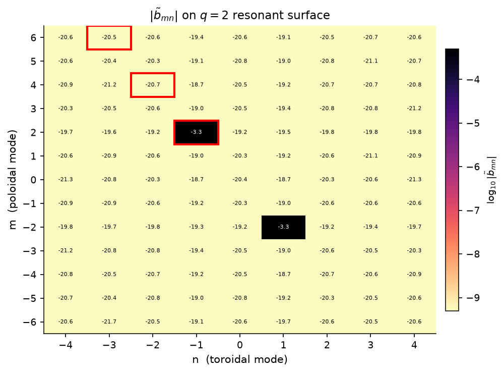
We compute the full \((m,n)\) Fourier spectrum of the divergence-free RMP template on the primary resonant surface. The resonant mode \((2,-1)\) and its driven harmonics are highlighted; the mixed-spectrum section above is the companion view that classifies resonant and non-resonant rows by detuning.
[13]:
psi_res_21 = eq.resonant_psi(2, 1)[0]
print(f'Computing (m,n) spectrum on q=2 surface (psi={psi_res_21:.3f}), n_theta=48, n_phi=48...')
b_mn = compute_mn_spectrum(
    delta_B_RMP,
    S=psi_res_21,
    equilibrium=eq,
    m_max=6,
    n_max=4,
    n_theta=48,
    n_phi=48,
)
print(f'Spectrum shape: {b_mn.shape}')

fig_sp, ax_sp = plt.subplots(figsize=(7, 5))
plot_mn_heatmap(
    b_mn, m_max=6, n_max=4,
    ax=ax_sp,
    log_scale=True,
    title=r'$|\tilde{b}_{mn}|$ on $q=2$ resonant surface',
    cmap='magma_r',
    highlight_modes=[(2, -1), (4, -2), (6, -3)],
)
plt.tight_layout()
plt.show()
Computing (m,n) spectrum on q=2 surface (psi=0.167), n_theta=48, n_phi=48...
Spectrum shape: (13, 9)
[MAGNETIC_SPECTRUM_ATLAS] Multi-component \(B^r\) spectrum atlas#
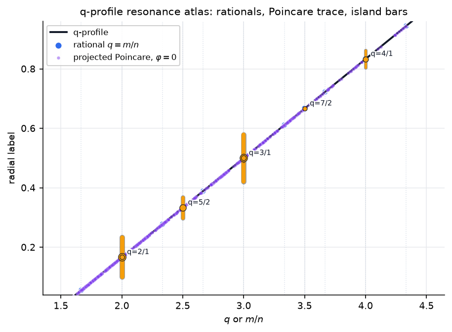
The single-surface heatmap above is useful for checking a dominant RMP row, but production magnetic-topology analysis usually needs a family view. Here we build a divergence-free multi-component perturbation, compute the Nardon-style contravariant radial spectrum \(\tilde b^1_{mn}=\delta B^1/B_0^3\) on a radial stack, and analyze all requested resonant rows together.
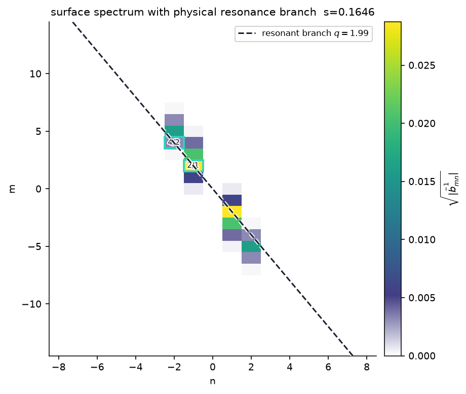
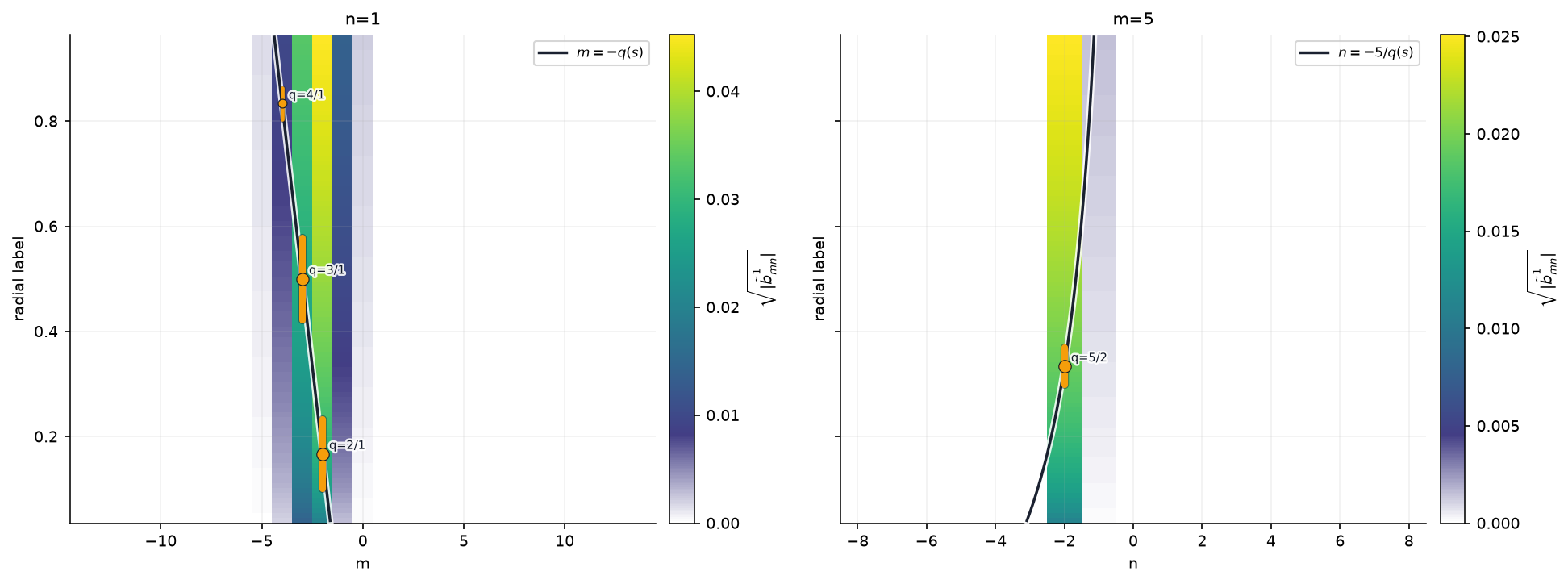
The utilities below are intentionally modular. The displayed atlas uses a wider signed Fourier window, 97 radial surfaces, amplitude_scale='sqrt', and white masks for zero/missing rows. The non-log colormap starts from the same white baseline, so near-zero coefficients do not look artificially separated from masked background. Signed axes show the actual Fourier rows in the computed spectrum: (m,n) is conjugate to (-m,-n) for a real field, but (m,n) and (m,-n) are independent
opposite-helicity rows unless the perturbation model imposes an extra symmetry. amplitude_scale='log10' remains useful when the goal is strict dynamic-range auditing rather than visual pattern recognition.
plot_rational_surface_mapcomposes optional q-profile, low-order rational markers, projected Poincare points, and island-width bars in the(m/n, s)plane.plot_spectrum_heatmap(..., renderer='pcolormesh')is the recommended surface-spectrum view; it can overlay the physical resonant branchm=-q n_Fwithout drawing the opposite-helicity branch.plot_spectrum_bar3dreturns an interactive Plotly figure for rotation, zoom, and hover inspection of dominant rows.plot_radial_mode_heatmap(fixed_n=..., resonant_sign=+1)follows all \(m\) rows at fixed Fourier \(n\) and draws the positive-q branch in the negative-\(m\) half-plane, \(m=-nq(s)\).plot_radial_mode_heatmap(fixed_m=..., axis_convention='fourier')follows actual Fourier \(n\) rows and draws the positive-q branch \(n=-m/q(s)\); the q-curve and island-width bars remain independently toggleable.
Yellow vertical bars mark the single-coefficient Nardon half-width estimate at the low-order rational surface; their thickness scales with the resonant coefficient amplitude. They are an optional overlay, not part of the heatmap itself. Only the physically resonant curve is drawn on each radial map. The opposite-helicity branch is not a conjugate diagnostic and is intentionally not mirrored here. If several harmonics share the same reduced rational surface, the true finite-amplitude island width should be computed from the combined resonant Hamiltonian; the per-row bars are diagnostics, not that nonlinear summed width.
[14]:
delta_B_multi_rmp = compose_magnetic_perturbations(
    radial_rmp_field_template(2, 1, amplitude=5.0e-4, phase=0.00, axis_R=eq.R0),
    radial_rmp_field_template(3, 1, amplitude=2.4e-4, phase=0.55, axis_R=eq.R0),
    radial_rmp_field_template(5, 2, amplitude=1.6e-4, phase=-0.35, axis_R=eq.R0),
)

S_scan = np.linspace(0.04, 0.96, 97)
theta_spec = np.linspace(0.0, 2*np.pi, 160, endpoint=False)
phi_spec = np.linspace(0.0, 2*np.pi, 96, endpoint=False)

theta_grid = theta_spec[None, None, :]
phi_grid = phi_spec[:, None, None]
r_scan = eq.r0 * np.sqrt(S_scan)[None, :, None]
R_stack = eq.R0 + r_scan * np.cos(theta_grid)
Z_stack = r_scan * np.sin(theta_grid)
R_stack = np.repeat(R_stack, phi_spec.size, axis=0)
Z_stack = np.repeat(Z_stack, phi_spec.size, axis=0)
Phi_stack = phi_grid + np.zeros_like(R_stack)

dBR_stack, dBZ_stack, dBphi_stack = delta_B_multi_rmp(R_stack, Z_stack, Phi_stack)
Bphi0_stack = eq.B0 * eq.R0 / np.maximum(R_stack, 1.0e-12)
tilde_b1_grid = nardon_radial_perturbation(
    R_stack,
    Z_stack,
    phi_spec,
    theta_spec,
    dBR_stack,
    dBZ_stack,
    dBphi_stack,
    S_scan,
    denominator_B_phi=Bphi0_stack,
)
magnetic_spectrum = radial_perturbation_Fourier_spectrum(
    tilde_b1_grid,
    theta_spec,
    phi_spec,
    radial_labels=S_scan,
    m_max=14,
    n_max=8,
    min_amplitude=1.0e-14,
)
q_scan = eq.q_of_psi(S_scan)
n_scan = [1, 2, 3]
m_scan = {1: range(1, 9), 2: range(2, 13), 3: range(3, 15)}
chains_multi = analyze_resonant_island_chains_multi_n(
    magnetic_spectrum,
    q_scan,
    n_values=n_scan,
    m_values=m_scan,
    min_b_res=1.0e-8,
)

print(f'Radial spectrum: {S_scan.size} surfaces, {magnetic_spectrum.m.size} retained Fourier rows over |m|<=14, |n|<=8.')
print(f'Multi-RMP analysis found {len(chains_multi)} resonant island-chain estimates.')
print('{:>7} {:>9} {:>9} {:>12} {:>12} {:>10}'.format('(m,n)', 's_res', 'q_res', 'b_res', 'half_width', 'phase'))
for chain in sorted(chains_multi, key=lambda item: item.b_res, reverse=True)[:8]:
    print('({:>2d},{:>1d}) {:>9.4f} {:>9.4f} {:>12.3e} {:>12.3e} {:>9.1f}°'.format(
        chain.m, chain.n, chain.radial_label, chain.q, chain.b_res, chain.half_width, np.degrees(chain.phase)
    ))

review_root = PROJECT_ROOT if PROJECT_ROOT is not None else pathlib.Path.cwd()
review_dir = review_root / 'pyna_output/magnetic_spectrum_review'
review_dir.mkdir(parents=True, exist_ok=True)

poincare_trace = None
if 'R_cross_p0' in globals() and len(R_cross_p0):
    S_p0 = np.clip(((R_cross_p0 - eq.R0)**2 + Z_cross_p0**2) / eq.r0**2, 0.0, 1.0)
    q_p0 = eq.q_of_psi(S_p0)
    poincare_trace = PoincareRationalTrace(
        ratio=q_p0,
        radial_label=S_p0,
        label=r'projected Poincare, $\varphi=0$',
    )

fig_qmap, ax_qmap, rational_markers = plot_rational_surface_map(
    S_scan,
    q_scan,
    n_values=n_scan,
    m_values=m_scan,
    chains=chains_multi,
    poincare=poincare_trace,
    show_poincare=poincare_trace is not None,
    max_island_bars=12,
    annotate_rationals=False,
    title='q-profile resonance atlas: rationals, Poincare trace, island bars',
)
fig_qmap.savefig(review_dir / '01_q_profile_resonance_map.png', dpi=180, bbox_inches='tight', facecolor='white')
plt.show()

surface_index = int(np.argmin(np.abs(S_scan - psi_res_21)))
surface_label = float(S_scan[surface_index])
chains_surface = [chain for chain in chains_multi if abs(chain.radial_label - surface_label) <= 0.08]
fig_surface, ax_surface = plt.subplots(figsize=(6.7, 5.7))
plot_spectrum_heatmap(
    magnetic_spectrum,
    radial_index=surface_index,
    m_values=np.arange(-14, 15),
    n_values=np.arange(-8, 9),
    chains=chains_surface,
    q_value=float(q_scan[surface_index]),
    renderer='pcolormesh',
    amplitude_scale='sqrt',
    mask_zeros=True,
    ax=ax_surface,
    cmap='viridis',
    title='surface spectrum with physical resonance branch',
)
fig_surface.savefig(review_dir / '02_surface_pcolormesh_atlas.png', dpi=180, bbox_inches='tight', facecolor='white')
plt.show()

fig_bar3d = plot_spectrum_bar3d(
    magnetic_spectrum,
    radial_index=surface_index,
    m_values=np.arange(-10, 11),
    n_values=np.arange(-6, 7),
    amplitude_scale='sqrt',
    range_mode='nonzero',
    bar_width=0.9,
    z_aspect=0.72,
    title='interactive 3D spectrum bars',
)
fig_bar3d.write_html(str(review_dir / '04_surface_plotly_bar3d.html'), include_plotlyjs='cdn')
try:
    fig_bar3d.write_image(str(review_dir / '04_surface_plotly_bar3d.png'), width=1040, height=650, scale=2)
except Exception as exc:
    print(f'Plotly static PNG export skipped: {exc}')
fig_bar3d.show()

fig_radial, axes_radial = plt.subplots(1, 2, figsize=(13.2, 4.9), sharey=True)
plot_radial_mode_heatmap(
    magnetic_spectrum,
    fixed_n=1,
    mode_values=np.arange(-14, 15),
    resonant_sign=1,
    q_profile=q_scan,
    chains=chains_multi,
    renderer='pcolormesh',
    amplitude_scale='sqrt',
    mask_zeros=True,
    ax=axes_radial[0],
    cmap='viridis',
    title='n=1',
)
plot_radial_mode_heatmap(
    magnetic_spectrum,
    fixed_m=5,
    mode_values=np.arange(-8, 9),
    axis_convention='fourier',
    q_profile=q_scan,
    chains=chains_multi,
    renderer='pcolormesh',
    amplitude_scale='sqrt',
    mask_zeros=True,
    ax=axes_radial[1],
    cmap='viridis',
    title='m=5',
)
plt.tight_layout()
fig_radial.savefig(review_dir / '03_radial_fixed_n_fixed_m_maps.png', dpi=180, bbox_inches='tight', facecolor='white')
plt.show()
Radial spectrum: 97 surfaces, 22 retained Fourier rows over |m|<=14, |n|<=8.
Multi-RMP analysis found 7 resonant island-chain estimates.
  (m,n)     s_res     q_res        b_res   half_width      phase
( 2,1)    0.1667    2.0000    1.661e-03    6.655e-02       0.6°
( 3,1)    0.5000    3.0000    1.535e-03    7.836e-02      27.6°
( 5,2)    0.3333    2.5000    7.401e-04    3.512e-02     -20.1°
( 4,1)    0.8333    4.0000    1.665e-04    2.980e-02      30.1°
( 6,2)    0.5000    3.0000    6.400e-05    1.131e-02     -20.1°
( 4,2)    0.1667    2.0000    2.132e-05    5.332e-03     -20.1°
( 7,2)    0.6667    3.5000    1.742e-06    2.016e-03     -20.1°
Data type cannot be displayed: application/vnd.plotly.v1+json
[PUBLICATION_FIGURE] Multi-phi 6-panel figure#
The same section helper scales to a compact multi-section layout. The O/X markers, O-point island-width bars, and local stable branches rotate with toroidal angle, while the PEST-style grid keeps the coordinate meaning visible in every panel.
[15]:
fig_pub, axes_pub = plot_rmp_resonance_sections(
    all_sections_data,
    phi_sections,
    eq=eq,
    components=components,
    colors=ISLAND_CMAPS,
    ncols=3,
    figsize=(12.0, 7.0),
    point_size=1.6,
    point_alpha=0.42,
    compact=True,
    overlays=('pest_grid', 'poincare', 'resonant_surfaces', 'stable_branches', 'island_width_bars', 'xo'),
    title=(
        'Stellarator RMP resonance: Poincare points, X/O geometry, '
        'island-width bars, stable branches, and PEST-style grid'
    ),
)

out_path = pathlib.Path('pyna_output/rmp_resonance_publication.png')
out_path.parent.mkdir(exist_ok=True)
fig_pub.savefig(str(out_path), dpi=170, bbox_inches='tight', facecolor='white')
print(f'Saved publication figure to {out_path}')
from IPython.display import display
display(fig_pub)
plt.close(fig_pub)
Saved publication figure to pyna_output/rmp_resonance_publication.png