Quick Start#
This page walks you through the three core capabilities of pyna — field-line tracing, Poincaré maps, and island topology — using a simple analytic tokamak equilibrium that requires no external data files.
Note
All examples use the Solov’ev analytic equilibrium (Cerfon & Freidberg 2010), scaled to EAST-like parameters (R₀ ≈ 1.86 m, B₀ = 5.3 T). It is a good all-purpose test bed: exact Grad–Shafranov solution, closed-form field components, adjustable shape.
1. Build an Analytic Equilibrium#
Start by importing the equilibrium and inspecting its basic parameters:
import numpy as np
import matplotlib.pyplot as plt
from pyna.toroidal.equilibrium import solovev_iter_like

eq = solovev_iter_like(scale=0.3)          # EAST-like size
Rmaxis, Zmaxis = eq.magnetic_axis

print(f"R0 = {eq.R0:.2f} m   a = {eq.a:.2f} m   B0 = {eq.B0:.1f} T")
print(f"κ  = {eq.kappa:.2f}  δ = {eq.delta:.2f}  q0 = {eq.q0:.2f}")
print(f"Magnetic axis: R = {Rmaxis:.3f} m, Z = {Zmaxis:.3f} m")
The returned eq object exposes eq.BR_BZ(R, Z), eq.Bphi(R),
eq.psi(R, Z) (normalised flux), and eq.q_profile(psi).
2. Trace Field Lines and Accumulate Poincaré Crossings#
A Poincaré section records the (R, Z) coordinates each time a field line crosses a chosen toroidal section (here φ = 0). After many toroidal turns, nested flux surfaces appear as closed curves; a magnetic island shows up as a chain of discrete section points.
from pyna.flt import FieldLineTracer, get_backend
from pyna.topo.poincare import PoincareAccumulator, poincare_from_fieldlines
from pyna.topo.section import ToroidalSection

# Use the canonical topology section type; ``pyna.topo.poincare`` keeps
# backward-compatible aliases for accumulator-only workflows.
section = ToroidalSection(0.0)

# --- define the ODE right-hand side: dR/dφ, dZ/dφ ---
def field_rhs(phi, RZ):
    R, Z = RZ
    BR, BZ = eq.BR_BZ(R, Z)
    Bphi   = eq.Bphi(R)
    return [R * BR / Bphi, R * BZ / Bphi]

# --- seed 8 field lines radially outward from the axis ---
R_starts = np.linspace(Rmaxis + 0.05, Rmaxis + 0.45, 8)
Z_starts = np.zeros(8)

# --- integrate 300 toroidal turns per line ---
backend = get_backend('cpu')
flt = FieldLineTracer(field_rhs, backend=backend)
pacc = poincare_from_fieldlines(
    field_func=field_rhs,
    start_pts=np.column_stack([R_starts, Z_starts, np.zeros_like(R_starts)]),
    sections=[section],
    t_max=300 * 2 * np.pi,
    backend=flt,
)
poincare_pts = [pacc.crossing_array(0)[:, :2]]

# --- plot ---
fig, ax = plt.subplots(figsize=(6, 6))
for Rs, Zs in poincare_pts:
    ax.scatter(Rs, Zs, s=0.8, color='steelblue')
ax.set_xlabel('R (m)')
ax.set_ylabel('Z (m)')
ax.set_aspect('equal')
ax.set_title('Poincaré map — Solov\'ev equilibrium')
plt.tight_layout()
plt.show()
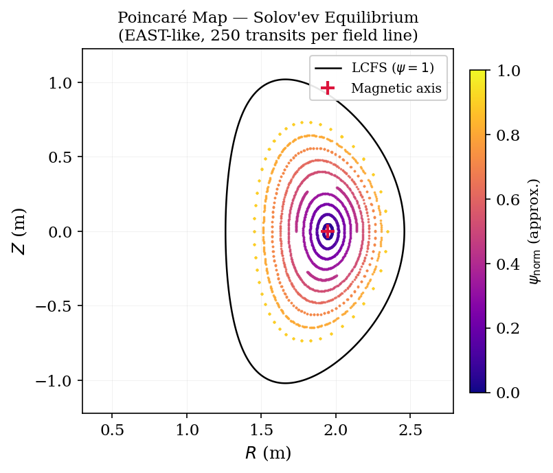
Figure 1. Poincaré map of the Solov’ev analytic equilibrium (EAST-like parameters, 250 toroidal transits per field line). Each colour corresponds to one field line; nested closed curves are flux surfaces. The red cross marks the magnetic axis; the black curve is the last closed flux surface (LCFS, ψ = 1).#
Each concentric ring corresponds to one field line winding around a flux surface. The q = m/n rational surface is where a resonant perturbation (e.g. an RMP coil) can open a magnetic island.
3. Locate a Rational Surface and Measure an Island#
After adding a small resonant perturbation, a magnetic island opens at the q = 2/1 surface. pyna can locate the surface and measure the island half-width in a single call:
from pyna.topo.toroidal_island import locate_rational_surface, island_halfwidth

# Build q(S) from PEST mesh
from pyna.toroidal.coords import build_PEST_mesh

nR, nZ = 100, 100
R_grid = np.linspace(0.3*eq.R0, 1.5*eq.R0, nR)
Z_grid = np.linspace(-eq.a*eq.kappa*1.3, eq.a*eq.kappa*1.3, nZ)
Rg, Zg  = np.meshgrid(R_grid, Z_grid, indexing='ij')

BR, BZ   = eq.BR_BZ(Rg, Zg)
Bphi     = eq.Bphi(Rg)
psi_norm = eq.psi(Rg, Zg)

S, TET, R_mesh, Z_mesh, q_iS = build_PEST_mesh(
    R_grid, Z_grid, BR, BZ, Bphi, psi_norm,
    Rmaxis, Zmaxis, ns=40, ntheta=181
)
S_values = S[1:]
q_values = q_iS[1:]
print(f"q range: {q_values[0]:.2f} → {q_values[-1]:.2f}")

# Locate q = 2/1 surface
res = locate_rational_surface(S_values, q_values, m=2, n=1)
print(f"q=2/1 surface at S = {res[0]:.4f}  (ψ_norm = {res[0]**2:.4f})")
The returned S_res value (S = √ψ_norm) tells you exactly where the
resonant layer sits. Pass it to island_halfwidth together with the
perturbed Poincaré map to get the island width in metres.
4. General Finite-Dimensional Dynamics#
pyna is not limited to toroidal field lines. The same topology object model is available for Hamiltonian systems, N-body flows, maps and SDE sample paths.
import numpy as np
from pyna.dynamics import (
    SeparableHamiltonianSystem,
    CallableMap,
    GeometricBrownianMotion,
)

oscillator = SeparableHamiltonianSystem(
    kinetic=lambda p, t: 0.5 * np.dot(p, p),
    potential=lambda q, t: 0.5 * np.dot(q, q),
    grad_kinetic=lambda p, t: p,
    grad_potential=lambda q, t: q,
    dof=1,
)
traj = oscillator.trajectory([1.0, 0.0], (0.0, 2*np.pi), dt=0.01)
print(traj.final)  # TimeSeriesSolution is a pyna.topo.core.Trajectory

linear_map = CallableMap(lambda x: np.array([2*x[0], 0.5*x[1]]), dim=2)
orbit = linear_map.orbit_geometry([1.0, 1.0], n_iter=5)
print(orbit.period_guess)

gbm = GeometricBrownianMotion(mu=[0.08], sigma=[0.2])
print(gbm.expected_log_growth())
Use pyna.topo.core objects such as Cycle, PeriodicOrbit,
Tube and IslandChain when a trajectory or map orbit has been promoted
from sampled data into a geometric/topological object.
5. Workflow-Based Construction#
For larger projects and teaching notebooks, use TopologyWorkflow to keep the
analysis sequence explicit without scattering ad-hoc constructors through the
code.
import numpy as np
from pyna.topo import TopologyWorkflow
from pyna.topo.section import HyperplaneSection

wf = TopologyWorkflow(closure_tol=1e-3)
flow = wf.system(
    "callable-flow",
    rhs=lambda x, t: np.array([x[1], -x[0]]),
    dim=2,
    coordinate_names=("q", "p"),
)

section = HyperplaneSection(np.array([1.0, 0.0]), 0.0, phase_dim=2)
pmap = wf.poincare_map(flow, section, dt=0.02)

closed_traj = wf.trajectory(flow, [1.0, 0.0], (0.0, 2*np.pi), dt=0.01)
cycle = wf.closed_cycle(closed_traj)
The lower-level adapters, builders, bridges and factories remain available for library authors, but most notebooks should start with the workflow facade.
6. Next Steps#
Tutorials — worked examples with plots: Mini Cases, SDE Monte Carlo Distributions, RMP Stellarator Resonance Analysis, Magnetic Coordinate Systems in Tokamak Equilibria, RMP Island Width Validation – Solov’ev Analytic Equilibrium
API reference — full docstrings: API Reference
CUDA acceleration — install
cupy-cuda12xand passbackend=get_backend('cuda')to the tracer for 100× speed-up on island-width scans.