RMPによるステラレータ共鳴解析#
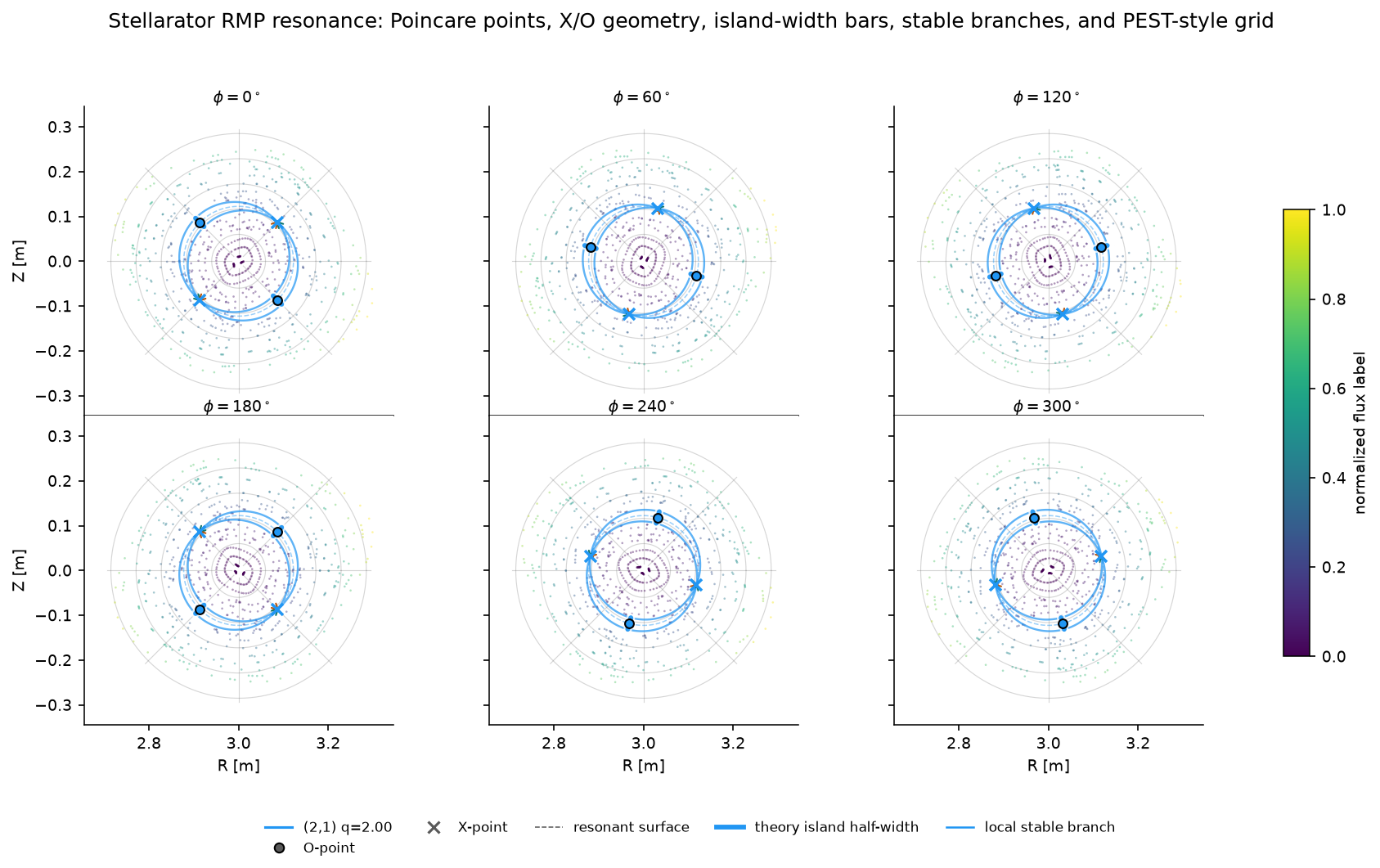
このノートブックは、解析的ステラレータ共鳴幾何の主要な公開ワークフローです。以前は別々だったテキストのみの 2 つのチュートリアルを、1 つの可視計算に統合しています。
解析的ステラレータ平衡を構築し、Poincaré断面を追跡する。
共鳴 RMP Fourier 成分と、その解析的な X/O 固定点を計算する。
生の断面点を幾何へ昇格する:交差点、固定点マーカー、共鳴面、O-point の島幅バー、局所安定枝、座標の重ね描き。
非摂動断面と摂動断面を PEST 風格子で比較する。
島幅、Chirikov オーバーラップ、\((m,n)\) スペクトルを要約する。
pyna.plotヘルパーを使って、現代的な多断面図を生成する。
このノートブックは、docs 公開前にローカルで実行することを前提にしています。GitHub Pages は磁力線追跡を再計算せず、保存済み出力を描画します。
[SETUP] import と公開用スタイル#
[1]:
import sys
import json
import pathlib
import numpy as np
import matplotlib
import matplotlib.pyplot as plt
from matplotlib.colors import Normalize

PROJECT_ROOT = None
for candidate in [pathlib.Path.cwd(), *pathlib.Path.cwd().parents]:
    if (candidate / 'pyna').is_dir() and (candidate / 'pyproject.toml').exists():
        PROJECT_ROOT = candidate
        break
if PROJECT_ROOT is not None and str(PROJECT_ROOT) not in sys.path:
    sys.path.insert(0, str(PROJECT_ROOT))

%matplotlib inline
from matplotlib_inline.backend_inline import set_matplotlib_formats
set_matplotlib_formats('png')

plt.rcParams.update({
    'font.family': 'DejaVu Sans',
    'font.size': 9,
    'axes.labelsize': 9,
    'axes.titlesize': 10,
    'figure.dpi': 150,
    'text.usetex': False,
    'axes.linewidth': 0.75,
    'axes.spines.top': False,
    'axes.spines.right': False,
    'figure.facecolor': 'white',
    'axes.facecolor': 'white',
})

from pyna.toroidal.equilibrium.stellarator import simple_stellarator
from pyna.toroidal.visual.RMP_spectrum import (
    find_resonant_components_analytic,
    radial_rmp_field_template,
    compose_magnetic_perturbations,
    circular_shell_divergence_diagnostic,
    fieldline_velocity_spectrum_on_circular_surface,
    rmp_nrmp_mode_rows,
    sample_stellarator_cylindrical_field,
    compare_cyna_fixed_points_for_component,
    deformed_circular_section_rz,
    deformed_surface_map_residual,
    project_fixed_points_to_deformed_surface,
    CoupledFixedPointSweep,
    plot_perturbation_order_summary,
    scan_nonresonant_residual_order,
    scan_coupled_fixed_point_sweep,
    scan_rmp_amplitude_order,
    scan_rmp_phase_order,
    scan_rmp_resolution_convergence,
    compute_mn_spectrum,
    plot_mn_heatmap,
    ISLAND_CMAPS,
)
from pyna.toroidal.perturbation_spectrum import (
    analyze_resonant_island_chains_multi_n,
    nardon_radial_perturbation,
    radial_perturbation_Fourier_spectrum,
)
from pyna.toroidal.visual.magnetic_spectrum import (
    PoincareRationalTrace,
    plot_radial_mode_heatmap,
    plot_rational_surface_map,
    plot_spectrum_bar3d,
    plot_spectrum_heatmap,
)
from pyna.topo.poincare import poincare_from_fieldlines, ToroidalSection
from pyna.plot import (
    draw_pest_grid,
    draw_poincare_points,
    draw_rmp_resonance_section,
    plot_rmp_resonance_sections,
)

print('Setup complete. numpy', np.__version__, '  matplotlib', matplotlib.__version__)
Setup complete. numpy 2.4.6 matplotlib 3.11.0
[EQ] ステラレータ平衡の構築#
次の単一ヘリシティの解析的ステラレータを使います。
大半径 \(R_0 = 3.0\) m、小半径 \(r_0 = 0.3\) m、軸上磁場 \(B_0 = 2.5\) T
線形 \(q\) プロファイル:\(q_0=1.5\)(軸)→ \(q_1=4.5\)(LCFS)
ヘリカルリップル:\((m_h, n_h) = (3,3)\)、\(\epsilon_h = 0.03\)
安全係数プロファイル \(q(\psi) = q_0 + (q_1-q_0)\psi\) は \([1.5, 4.5]\) を覆うため、\(q = 2/1, 3/1, 4/1\) などの共鳴がプラズマ内に存在します。
[2]:
eq = simple_stellarator(
    R0=3.0, r0=0.3, B0=2.5,
    q0=1.5, q1=4.5,
    m_h=3, n_h=3, epsilon_h=0.03,
)
print(eq)
print(f'q range: [{eq.q0}, {eq.q1}]')
print(f'Resonant surface for (2,1): psi_res = {eq.resonant_psi(2,1)}')
print(f'Resonant surface for (4,2): psi_res = {eq.resonant_psi(4,2)}')
print(f'Resonant surface for (6,3): psi_res = {eq.resonant_psi(6,3)}')

# Convenience references
R0_eq = eq.R0
r0_eq = eq.r0
StellaratorSimple(R0=3.0 m, r0=0.3 m, B0=2.5 T, q=[1.5, 4.5], m_h=3, n_h=3, ε_h=0.03)
q range: [1.5, 4.5]
Resonant surface for (2,1): psi_res = [0.16666666666666666]
Resonant surface for (4,2): psi_res = [0.16666666666666666]
Resonant surface for (6,3): psi_res = [0.16666666666666666]
[RMP_NRMP_WORKFLOW] RMP/nRMP分解#
磁束面上の摂動モードは、局所的な磁力線回転と比較して初めて有用になります。Fourier 規約を
とすると、局所離調は
成分 |
条件 |
幾何的効果 |
pyna ワークフロー |
|---|---|---|---|
RMP |
|
磁気島列を開く;X/O 点、O-point 島幅バー、セパラトリクス枝が一次オブジェクトとして意味を持つ |
|
nRMP |
すべての非共鳴モードで |
すべての非共鳴モードが滑らかな磁束面変形と磁力線速度変調に寄与する |
|
混合スペクトル |
両方が存在 |
共鳴磁気島幾何は、合計 nRMP 変形を受けた面の上に載る |
|
検証 |
ベクトル場が物理的であること |
非ソレノイダルなテンプレートは偽のトポロジーを作り得る |
|
重要な違いは、RMP 診断が共鳴行に注目するのに対し、nRMP 応答はすべての非共鳴行にわたる完全な和であることです。
寄与表はランキングと収束確認には有用ですが、モデルは選んだ上位成分ではなく、完全な非共鳴スペクトルです。
[POINCARE_UNPERTURBED] phi=0 の非摂動 Poincaré断面#
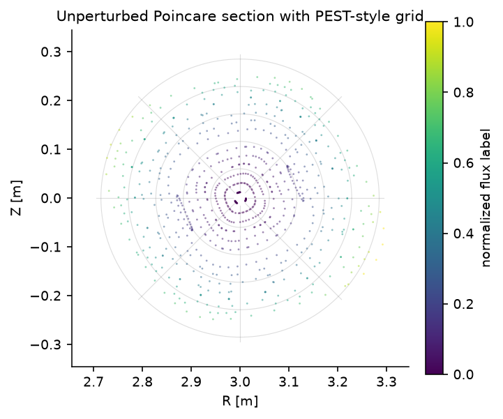
非摂動平衡の磁力線を追跡し、\(\varphi=0\) 平面での交差点を記録します。結果は生のサンプリングされた幾何であり、有用ではありますが、まだトポロジーオブジェクトではありません。後続セルでは、共鳴面、X/O マーカー、局所安定枝、PEST 風座標格子を重ねることで昇格レイヤーを追加します。
交差点は pyna_output/poincare_unperturbed.json にキャッシュされます。
[3]:
CACHE_UNPERT = pathlib.Path('pyna_output/poincare_unperturbed.json')
CACHE_UNPERT.parent.mkdir(exist_ok=True)

if CACHE_UNPERT.exists():
    _d = json.loads(CACHE_UNPERT.read_text())
    R_cross_u = np.array(_d['R'])
    Z_cross_u = np.array(_d['Z'])
    print(f'Loaded from cache: {len(R_cross_u)} crossings')
else:
    n_fieldlines = 15
    n_turns = 50
    dt = 0.08
    t_max = n_turns * 2 * np.pi * eq.R0

    R_starts = np.linspace(eq.R0 + 0.04*eq.r0, eq.R0 + 0.92*eq.r0, n_fieldlines)
    start_pts = np.zeros((n_fieldlines, 3))
    start_pts[:, 0] = R_starts
    start_pts[:, 2] = 0.0

    sections_u = [ToroidalSection(phi0=0.0)]
    print(f'Tracing {n_fieldlines} field lines x {n_turns} turns (dt={dt}, t_max={t_max:.1f} m)...')

    pmap_u = poincare_from_fieldlines(
        eq.field_func,
        start_pts,
        sections_u,
        t_max=t_max,
        dt=dt,
    )
    arr_u = pmap_u.crossing_array(0)
    R_cross_u = arr_u[:, 0]
    Z_cross_u = arr_u[:, 1]
    print(f'Computed: {len(R_cross_u)} crossings. Caching...')
    CACHE_UNPERT.write_text(json.dumps({'R': R_cross_u.tolist(), 'Z': Z_cross_u.tolist()}))
    print('Cached.')

fig_u, ax_u = plt.subplots(figsize=(4.7, 4.3), constrained_layout=True)
draw_pest_grid(ax_u, eq, alpha=0.22)
psi_pts = np.clip(((R_cross_u - eq.R0)**2 + Z_cross_u**2) / eq.r0**2, 0, 1)
draw_poincare_points(
    ax_u,
    R_cross_u,
    Z_cross_u,
    values=psi_pts,
    cmap='viridis',
    point_size=1.8,
    alpha=0.50,
    rasterized=False,
)
sm_u = plt.cm.ScalarMappable(cmap='viridis', norm=Normalize(0, 1))
fig_u.colorbar(sm_u, ax=ax_u, label='normalized flux label', shrink=0.82)
lim = 1.15 * eq.r0
ax_u.set_xlim(eq.R0 - lim, eq.R0 + lim)
ax_u.set_ylim(-lim, lim)
ax_u.set_aspect('equal')
ax_u.set_xlabel('R [m]')
ax_u.set_ylabel('Z [m]')
ax_u.set_title('Unperturbed Poincare section with PEST-style grid')
plt.show()
Loaded from cache: 735 crossings
[RMP_FIELD] RMP 摂動場の定義と可視化#
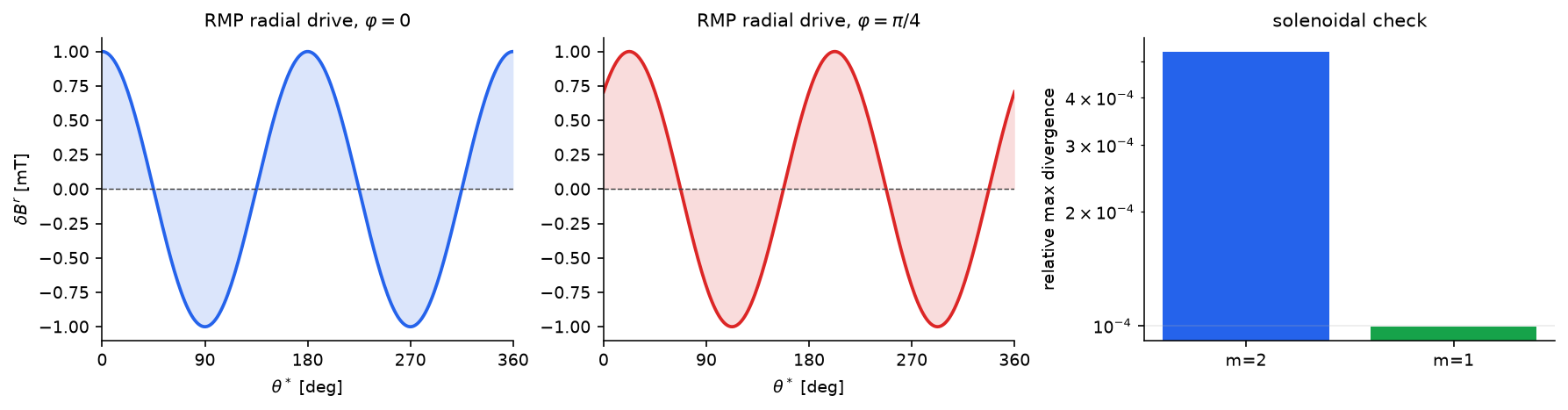
基本モード \((m,n)=(2,1)\)、振幅 \(\delta B=1\) mT の単一モード RMP を加えます。ユーザーに見えるテンプレートは
ですが、radial_rmp_field_template は、局所円筒シェル計量で完全な円筒座標ベクトル場を発散なしにするために必要な補償ポロイダル/トロイダル成分も追加します。描画される径方向射影は、従来どおりの共鳴駆動 \(\delta B^r\) です。
同じヘルパーは重要な m=1 分枝もサポートします。この場合は、径方向発散に theta 非依存部分が含まれるため、トロイダル成分が必要です。
[4]:
base_m, base_n = 2, 1
B_rmp = 1e-3  # 1 mT

delta_B_RMP = radial_rmp_field_template(
    base_m,
    base_n,
    amplitude=B_rmp,
    phase=0.0,
    axis_R=eq.R0,
)

psi_res_21 = eq.resonant_psi(2, 1)[0]
r_res_21 = np.sqrt(psi_res_21) * eq.r0
print(f'q=2/1 resonant surface: psi={psi_res_21:.3f}, r={r_res_21*100:.1f} cm')
print(f'delta_B/B0 = {B_rmp/eq.B0*100:.3f}%')

r_check = np.linspace(0.08, 0.28, 7)
div_m2 = circular_shell_divergence_diagnostic(
    delta_B_RMP,
    axis_R=eq.R0,
    r_values=r_check,
    n_theta=192,
    n_phi=192,
)
delta_B_m1_demo = radial_rmp_field_template(
    1,
    1,
    amplitude=B_rmp,
    phase=0.35,
    axis_R=eq.R0,
)
div_m1 = circular_shell_divergence_diagnostic(
    delta_B_m1_demo,
    axis_R=eq.R0,
    r_values=r_check,
    n_theta=192,
    n_phi=192,
)

print('Divergence diagnostics for the full vector perturbation:')
print('{:<8} {:>12} {:>12} {:>12}'.format('mode', 'max |div|', 'rms |div|', 'rel max'))
for label, diag in [('m=2', div_m2), ('m=1', div_m1)]:
    print(f'{label:<8} {diag.max_abs:12.3e} {diag.rms:12.3e} {diag.relative_max:12.3e}')

theta_arr = np.linspace(0, 2*np.pi, 240)
R_res = eq.R0 + r_res_21 * np.cos(theta_arr)
Z_res = r_res_21 * np.sin(theta_arr)

fig_rmp, axes_rmp = plt.subplots(1, 3, figsize=(11.8, 3.0), constrained_layout=True)
for ax, phi_val, phi_label, color in [
    (axes_rmp[0], 0.0, r'$\varphi=0$', '#2563eb'),
    (axes_rmp[1], np.pi/4, r'$\varphi=\pi/4$', '#dc2626'),
]:
    BR, BZ, _ = delta_B_RMP(R_res, Z_res, phi_val)
    dBpsi = BR*np.cos(theta_arr) + BZ*np.sin(theta_arr)
    ax.plot(np.degrees(theta_arr), dBpsi * 1e3, color=color, linewidth=1.8)
    ax.fill_between(np.degrees(theta_arr), 0, dBpsi * 1e3, color=color, alpha=0.16, linewidth=0)
    ax.axhline(0, color='0.25', lw=0.7, linestyle='--')
    ax.set_xlabel(r'$\theta^*$ [deg]')
    ax.set_title(f'RMP radial drive, {phi_label}')
    ax.set_xlim(0, 360)
    ax.set_xticks([0, 90, 180, 270, 360])
axes_rmp[0].set_ylabel(r'$\delta B^r$ [mT]')

axes_rmp[2].bar(['m=2', 'm=1'], [div_m2.relative_max, div_m1.relative_max], color=['#2563eb', '#16a34a'])
axes_rmp[2].set_yscale('log')
axes_rmp[2].set_ylabel('relative max divergence')
axes_rmp[2].set_title('solenoidal check')
axes_rmp[2].grid(True, axis='y', alpha=0.25)
plt.show()
print('Divergence-free RMP field defined and visualised.')
q=2/1 resonant surface: psi=0.167, r=12.2 cm
delta_B/B0 = 0.040%
Divergence diagnostics for the full vector perturbation:
mode        max |div|    rms |div|      rel max
m=2         6.642e-06    3.148e-06    5.300e-04
m=1         1.804e-06    7.949e-07    9.946e-05
Divergence-free RMP field defined and visualised.
[M1_RMP] m=1 位相制御ミニケース#
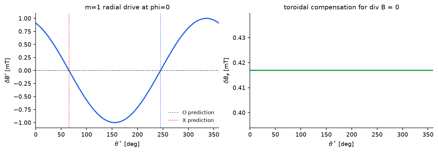
m=1 摂動は十分に一般的であり、特殊ケースとして扱うべきではありません。ここでは同じ発散なしテンプレートが、単純な q=1 平衡で (1,1) 共鳴を駆動します。短い計算で 3 点を検証します:場が数値的にソレノイダルであること、抽出した b_{1,-1} 位相がテンプレート位相に従うこと、予測された O/X 点が径方向駆動のゼロ交差上に来ることです。
[5]:
eq_m1 = simple_stellarator(
    R0=eq.R0,
    r0=eq.r0,
    B0=eq.B0,
    q0=0.75,
    q1=1.25,
    m_h=eq.m_h,
    n_h=eq.n_h,
    epsilon_h=0.0,
)
m1_phase = 0.43
delta_B_m1 = radial_rmp_field_template(
    1,
    1,
    amplitude=B_rmp,
    phase=m1_phase,
    axis_R=eq_m1.R0,
)
psi_res_m1 = eq_m1.resonant_psi(1, 1)[0]
r_res_m1 = np.sqrt(psi_res_m1) * eq_m1.r0
m1_diag = circular_shell_divergence_diagnostic(
    delta_B_m1,
    axis_R=eq_m1.R0,
    r_values=np.linspace(0.08, 0.28, 7),
    n_theta=192,
    n_phi=192,
)
component_m1 = find_resonant_components_analytic(
    eq_m1,
    delta_B_m1,
    base_m=1,
    base_n=1,
    max_harmonic=1,
    n_theta=128,
    n_phi=64,
    min_amplitude=1e-16,
)[0]

print(f'm=1 resonant surface: psi={psi_res_m1:.3f}, r={r_res_m1*100:.1f} cm')
print(f'arg b_(1,-1) = {np.angle(component_m1.b_mn):.6f} rad, template phase = {m1_phase:.6f} rad')
print(f'|b_(1,-1)| = {abs(component_m1.b_mn):.3e} T, expected about B_rmp/2 = {0.5*B_rmp:.3e} T')
print(f'm=1 divergence relative max = {m1_diag.relative_max:.3e}')
print(f'O-point theta = {np.degrees(component_m1.opoint_theta):.2f} deg')
print(f'X-point theta = {np.degrees(component_m1.xpoint_theta):.2f} deg')

theta_m1 = np.linspace(0, 2*np.pi, 361)
R_m1 = eq_m1.R0 + r_res_m1*np.cos(theta_m1)
Z_m1 = r_res_m1*np.sin(theta_m1)
BR_m1, BZ_m1, Bphi_m1 = delta_B_m1(R_m1, Z_m1, 0.0)
dBr_m1 = BR_m1*np.cos(theta_m1) + BZ_m1*np.sin(theta_m1)

fig_m1, (ax_m1, ax_m1b) = plt.subplots(1, 2, figsize=(9.4, 3.2), constrained_layout=True)
ax_m1.plot(np.degrees(theta_m1), dBr_m1*1e3, color='#2563eb', lw=1.8)
ax_m1.axhline(0, color='0.25', lw=0.7, ls='--')
ax_m1.axvline(np.degrees(component_m1.opoint_theta), color='#2563eb', lw=1.1, ls=':', label='O prediction')
ax_m1.axvline(np.degrees(component_m1.xpoint_theta), color='#dc2626', lw=1.1, ls=':', label='X prediction')
ax_m1.set_xlim(0, 360)
ax_m1.set_xlabel(r'$\theta^*$ [deg]')
ax_m1.set_ylabel(r'$\delta B^r$ [mT]')
ax_m1.set_title('m=1 radial drive at phi=0')
ax_m1.legend(frameon=False, fontsize=8)

ax_m1b.plot(np.degrees(theta_m1), Bphi_m1*1e3, color='#16a34a', lw=1.8)
ax_m1b.set_xlim(0, 360)
ax_m1b.set_xlabel(r'$\theta^*$ [deg]')
ax_m1b.set_ylabel(r'$\delta B_\varphi$ [mT]')
ax_m1b.set_title('toroidal compensation for div B = 0')
plt.show()
  k=1: (1,1) ψ_res=0.500 q_res=1.000 |b_mn|=5.000e-04 phase_arg=24.6° w_ψ=0.1265 (2.68 cm) θ_O=245.4° θ_X=65.4°
m=1 resonant surface: psi=0.500, r=21.2 cm
arg b_(1,-1) = 0.430000 rad, template phase = 0.430000 rad
|b_(1,-1)| = 5.000e-04 T, expected about B_rmp/2 = 5.000e-04 T
m=1 divergence relative max = 9.946e-05
O-point theta = 245.36 deg
X-point theta = 65.36 deg
[RESONANT_COMPONENTS] 共鳴 Fourier 成分の抽出#
2D FFT を使って各共鳴磁束面上の RMP 場を分解し、共鳴 \((m_k, n_k) = k\times(2,1)\) 高調波の振幅を抽出します。磁気島の半幅 は Rutherford 公式で与えられます。
結果は pyna_output/rmp_components.json にキャッシュされます。
[6]:
CACHE_COMP = pathlib.Path('pyna_output/rmp_components.json')
CACHE_COMP.parent.mkdir(exist_ok=True)

print('Computing resonant components (n_theta=32, n_phi=16)...')
components = find_resonant_components_analytic(
    eq, delta_B_RMP, base_m=base_m, base_n=base_n,
    max_harmonic=3, n_theta=32, n_phi=16,
)
print(f'Found {len(components)} resonant components.')

# Cache as JSON
_comp_data = [{
    'm': c.m, 'n': c.n, 'harmonic_order': c.harmonic_order,
    'b_mn_real': float(c.b_mn.real), 'b_mn_imag': float(c.b_mn.imag),
    'psi_res': float(c.psi_res), 'q_res': float(c.q_res),
    'half_width_psi': float(c.half_width_psi),
    'half_width_r': float(c.half_width_r),
    'opoint_theta': float(c.opoint_theta),
    'xpoint_theta': float(c.xpoint_theta),
    'q_prime_sign': int(c.q_prime_sign),
} for c in components]
CACHE_COMP.write_text(json.dumps(_comp_data, indent=2))
print('Cached to', CACHE_COMP)

# Print table
print()
print(f'{"k":>3}  {"(m,n)":>8}  {"psi_res":>8}  {"q_res":>6}  {"b_mn|":>10}  {"w_psi":>8}  {"w_r (cm)":>10}  {"theta_O":>8}  {"theta_X":>8}')
print('-'*80)
for c in components:
    print(f'{c.harmonic_order:>3}  ({c.m},{c.n}){"":>4}  {c.psi_res:>8.4f}  {c.q_res:>6.3f}  {abs(c.b_mn):>10.3e}  {c.half_width_psi:>8.4f}  {c.half_width_r*100:>10.2f}  {np.degrees(c.opoint_theta):>8.1f}  {np.degrees(c.xpoint_theta):>8.1f}')
Computing resonant components (n_theta=32, n_phi=16)...
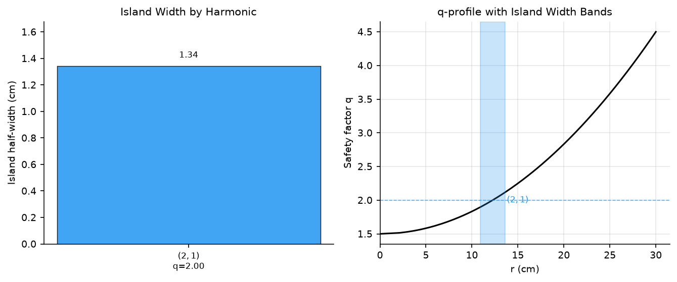
  k=1: (2,1) ψ_res=0.167 q_res=2.000 |b_mn|=5.000e-04 phase_arg=-0.0° w_ψ=0.0365 (1.34 cm) θ_O=135.0° θ_X=45.0°
  k=2: (4,2) — |b_mn|=4.57e-21 below threshold
  k=3: (6,3) — |b_mn|=1.98e-20 below threshold
Found 1 resonant components.
Cached to pyna_output/rmp_components.json

  k     (m,n)   psi_res   q_res       b_mn|     w_psi    w_r (cm)   theta_O   theta_X
--------------------------------------------------------------------------------
  1  (2,1)        0.1667   2.000   5.000e-04    0.0365        1.34     135.0      45.0
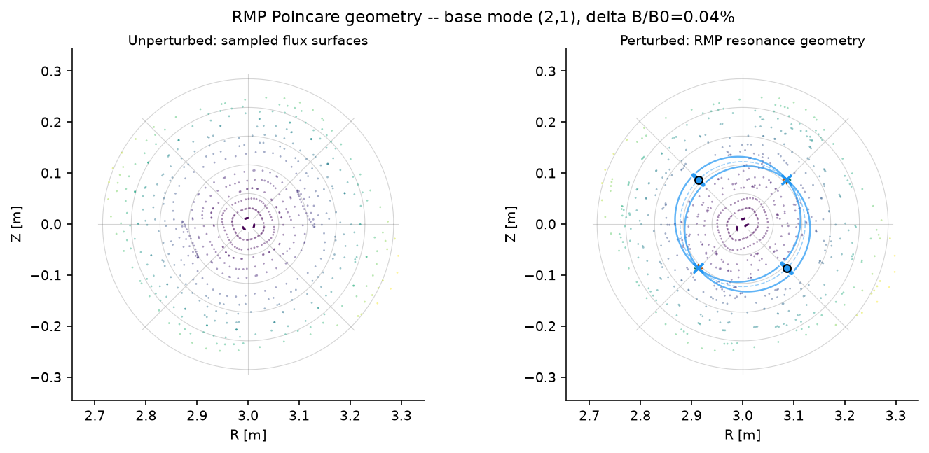
[POINCARE_PERTURBED] 幾何への昇格:交差点 -> X/O 点 -> 多様体#
摂動追跡はサンプリングされた Poincaré 点を与えます。解析的 RMP スペクトルは固定点と島幅の予測を与えます。pyna.plot.draw_rmp_resonance_section はこれらを 1 つの断面幾何にまとめます。
磁束ラベルで色分けした Poincaré 点;
PEST 風の \((S,\theta^*)\) 格子線;
各高調波の共鳴面;
解析的固定点公式から得た O-points と X-points;
共鳴 Fourier 振幅で長さが決まる O-point 径方向バー;
X-points から生じる局所安定セパラトリクス枝。
これは一般幾何ワークフローと同じ昇格の考え方です。明示的なモデルまたは診断が昇格を正当化するまで、生のサンプルは永続的な幾何オブジェクトや重ね描きから区別して保持されます。
[7]:
# Perturbed field_func
# --------------------
def field_func_perturbed(rzphi_1d):
    """Unit-tangent dRZphi/ds for the field-line ODE with RMP added."""
    rzphi_1d = np.asarray(rzphi_1d, dtype=float)
    R, Z, phi = rzphi_1d[0], rzphi_1d[1], rzphi_1d[2]
    theta = np.arctan2(Z, R - R0_eq)
    psi = eq.psi_ax(R, Z)
    q = float(eq.q_of_psi(psi))
    r_minor = np.sqrt((R - R0_eq)**2 + Z**2)
    B_phi = eq.B0 * eq.R0 / R
    B_pol = B_phi * r_minor / (R * max(abs(q), 1e-3))
    if r_minor > 1e-10:
        BR0 = -B_pol * np.sin(theta)
        BZ0 =  B_pol * np.cos(theta)
    else:
        BR0 = BZ0 = 0.0
    delta_BR_eq = eq.epsilon_h * eq.B0 * psi * np.cos(eq.m_h * theta - eq.n_h * phi)
    db = delta_B_RMP(R, Z, phi)
    BR_tot = BR0 + delta_BR_eq + db[0]
    BZ_tot = BZ0 + db[1]
    B_phi_tot = B_phi + db[2]
    B_mag = np.sqrt(BR_tot**2 + BZ_tot**2 + B_phi_tot**2) + 1e-30
    return np.array([BR_tot/B_mag, BZ_tot/B_mag, B_phi_tot/(R*B_mag)])

CACHE_PERT = pathlib.Path('pyna_output/poincare_perturbed_divfree.json')
CACHE_PERT.parent.mkdir(exist_ok=True)

phi_sections_deg = [0, 60, 120, 180, 240, 300]
phi_sections = np.array(phi_sections_deg) * np.pi / 180.0

if CACHE_PERT.exists():
    _d = json.loads(CACHE_PERT.read_text())
    all_sections_data = _d['sections']
    print(f'Loaded perturbed Poincare from cache ({len(all_sections_data)} sections).')
else:
    sections_p = [ToroidalSection(phi0=ph) for ph in phi_sections]
    n_fieldlines, n_turns, dt = 15, 50, 0.08
    t_max = n_turns * 2 * np.pi * eq.R0
    start_pts = np.zeros((n_fieldlines, 3))
    start_pts[:, 0] = np.linspace(eq.R0 + 0.04*eq.r0, eq.R0 + 0.92*eq.r0, n_fieldlines)

    print(f'Tracing {n_fieldlines} field lines x {n_turns} turns (t_max={t_max:.1f} m)...')
    pmap_p = poincare_from_fieldlines(field_func_perturbed, start_pts, sections_p, t_max=t_max, dt=dt)
    all_sections_data = []
    for i_sec, phi_deg in enumerate(phi_sections_deg):
        arr = pmap_p.crossing_array(i_sec)
        print(f'  phi={phi_deg} deg: {len(arr)} crossings')
        all_sections_data.append({'R': arr[:, 0].tolist() if len(arr) else [], 'Z': arr[:, 1].tolist() if len(arr) else []})
    CACHE_PERT.write_text(json.dumps({'phi_sections_deg': phi_sections_deg, 'sections': all_sections_data}))
    print('Computed and cached.')

R_cross_p0 = np.array(all_sections_data[0]['R'])
Z_cross_p0 = np.array(all_sections_data[0]['Z'])
print(f'phi=0 section: {len(R_cross_p0)} crossings')

fig2, (axL, axR) = plt.subplots(1, 2, figsize=(9.4, 4.2), constrained_layout=True)

# The low-level plot layers are independently selectable by name.
draw_rmp_resonance_section(
    axL,
    R_cross_u,
    Z_cross_u,
    eq=eq,
    components=[],
    phi=0.0,
    title='Unperturbed: sampled flux surfaces',
    overlays=('pest_grid', 'poincare'),
    point_size=1.8,
    point_alpha=0.46,
)
draw_rmp_resonance_section(
    axR,
    R_cross_p0,
    Z_cross_p0,
    eq=eq,
    components=components,
    phi=0.0,
    colors=ISLAND_CMAPS,
    title='Perturbed: RMP resonance geometry',
    overlays=('pest_grid', 'poincare', 'resonant_surfaces', 'stable_branches', 'island_width_bars', 'xo'),
    point_size=1.8,
    point_alpha=0.46,
)

fig2.suptitle(
    f'RMP Poincare geometry -- base mode ({base_m},{base_n}), '
    f'delta B/B0={B_rmp/eq.B0*100:.2f}%',
    fontsize=11,
)
plt.show()
Loaded perturbed Poincare from cache (6 sections).
phi=0 section: 735 crossings
[CYNA_FIXED_POINTS] Newton 固定点と RMP スペクトル位相の比較#
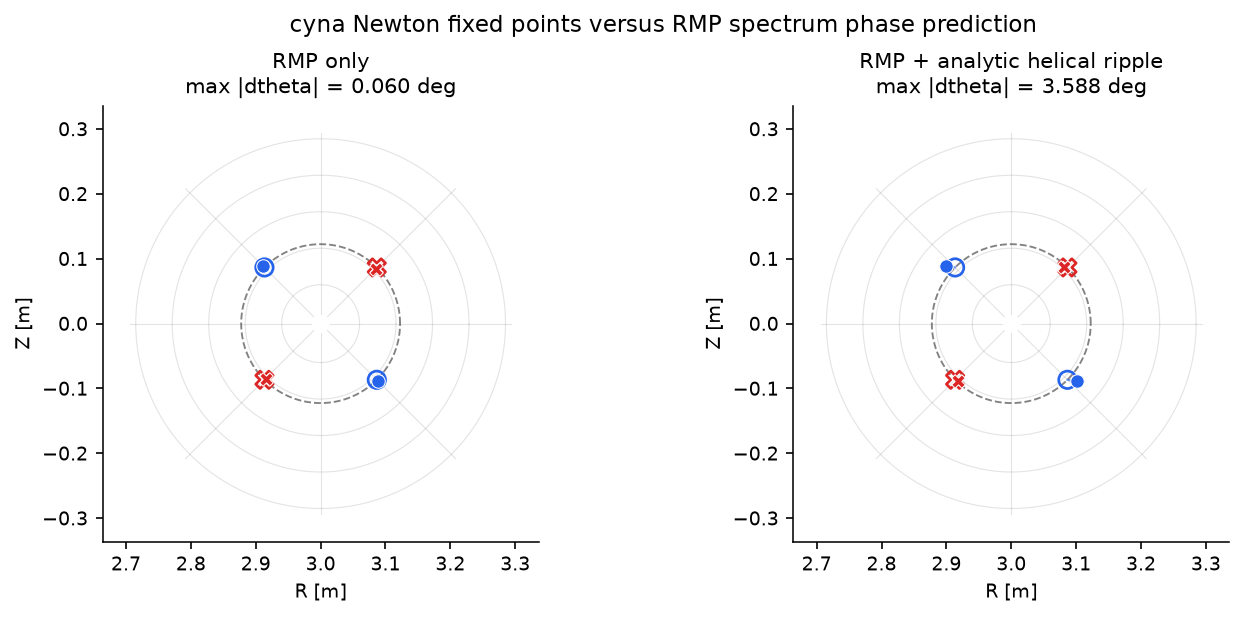
RMP スペクトルは一次の O/X 点位相を予測します。ここでは高速化された cyna Newton 写像を使い、それらの初期値を真の周期軌道固定点へ改良してから位相誤差を測定します。RMP のみのケースはコードの健全性確認です。解析的ヘリカルリップルを加えると、一次スペクトルが意図的に無視している有限振幅/モデルによるずれが見えます。
[8]:
# Build a physical cylindrical field for cyna and compare Newton fixed points.
def row_newton_theta_deg(row, eq_case):
    axis_R, axis_Z = eq_case.magnetic_axis
    theta = np.arctan2(row.newton_Z - axis_Z, row.newton_R - axis_R) % (2*np.pi)
    return float(np.degrees(theta))


cyna_rows_by_case = {}
cyna_eq_by_case = {}
if components:
    eq_rmp_only = simple_stellarator(
        R0=eq.R0, r0=eq.r0, B0=eq.B0,
        q0=eq.q0, q1=eq.q1,
        m_h=eq.m_h, n_h=eq.n_h, epsilon_h=0.0,
    )
    try:
        for case_label, eq_case in [
            ('RMP only', eq_rmp_only),
            ('RMP + analytic helical ripple', eq),
        ]:
            print(f'Building cyna field: {case_label}')
            field_case = sample_stellarator_cylindrical_field(
                eq_case,
                delta_B_RMP,
                nR=128,
                nPhi=128,
                label=f'analytic_rmp_for_cyna_{case_label.replace(" ", "_").lower()}',
            )
            rows = compare_cyna_fixed_points_for_component(
                field_case,
                components[0],
                eq_case,
                DPhi=0.015,
                max_iter=80,
                tol=1e-11,
                n_threads=4,
            )
            cyna_rows_by_case[case_label] = rows
            cyna_eq_by_case[case_label] = eq_case
    except ImportError as exc:
        print('cyna fixed-point comparison skipped:', exc)

if cyna_rows_by_case:
    print()
    header = '{:<30} {:>4} {:>6} {:>9} {:>9} {:>10} {:>11} {:>11} {:>11}'.format(
        'case', 'kind', 'branch', 'theta*', 'theta_N', 'dtheta', 'm*dtheta', 'dr [cm]', 'residual'
    )
    print(header)
    print('-' * len(header))
    for case_label, rows in cyna_rows_by_case.items():
        eq_case = cyna_eq_by_case[case_label]
        for row in rows:
            theta_n = row_newton_theta_deg(row, eq_case)
            print('{:<30} {:>4} {:>6d} {:>9.3f} {:>9.3f} {:>10.4f} {:>11.4f} {:>11.4f} {:>11.1e}'.format(
                case_label,
                row.predicted_kind + '/' + (row.newton_kind or '?'),
                row.branch,
                row.predicted_theta_deg,
                theta_n,
                row.theta_error_deg,
                row.helical_phase_error_deg,
                row.radial_error_cm,
                row.residual,
            ))
        max_dtheta = max(abs(row.theta_error_deg) for row in rows)
        max_helical = max(abs(row.helical_phase_error_deg) for row in rows)
        print(f'  -> {case_label}: max |dtheta|={max_dtheta:.4f} deg, max |m*dtheta|={max_helical:.4f} deg')

if cyna_rows_by_case:
    fig_cmp, axes_cmp = plt.subplots(1, len(cyna_rows_by_case), figsize=(9.2, 4.0), constrained_layout=True)
    axes_cmp = np.atleast_1d(axes_cmp)
    for ax, (case_label, rows) in zip(axes_cmp, cyna_rows_by_case.items()):
        eq_case = cyna_eq_by_case[case_label]
        draw_pest_grid(ax, eq_case, alpha=0.18)
        r_res = np.sqrt(components[0].psi_res) * eq_case.r0
        theta_ring = np.linspace(0, 2*np.pi, 361)
        ax.plot(eq_case.R0 + r_res*np.cos(theta_ring), r_res*np.sin(theta_ring),
                color='0.25', lw=0.9, ls='--', alpha=0.65)
        for row in rows:
            color = '#2563eb' if row.predicted_kind == 'O' else '#dc2626'
            marker = 'o' if row.predicted_kind == 'O' else 'X'
            ax.plot([row.predicted_R, row.newton_R], [row.predicted_Z, row.newton_Z],
                    color=color, lw=1.0, alpha=0.65)
            ax.scatter(row.predicted_R, row.predicted_Z, marker=marker, s=70,
                       facecolors='none', edgecolors=color, linewidths=1.3, zorder=5)
            ax.scatter(row.newton_R, row.newton_Z, marker=marker, s=42,
                       color=color, edgecolors='white', linewidths=0.5, zorder=6)
        lim = 1.12 * eq_case.r0
        ax.set_xlim(eq_case.R0 - lim, eq_case.R0 + lim)
        ax.set_ylim(-lim, lim)
        ax.set_aspect('equal')
        ax.set_xlabel('R [m]')
        ax.set_ylabel('Z [m]')
        max_dtheta = max(abs(row.theta_error_deg) for row in rows)
        ax.set_title(f'{case_label}\nmax |dtheta| = {max_dtheta:.3f} deg')
    fig_cmp.suptitle('cyna Newton fixed points versus RMP spectrum phase prediction', fontsize=11)
    plt.show()
Building cyna field: RMP only
Building cyna field: RMP + analytic helical ripple

case                           kind branch    theta*   theta_N     dtheta    m*dtheta     dr [cm]    residual
-------------------------------------------------------------------------------------------------------------
RMP only                        O/O      0   315.000   314.940    -0.0602     -0.1203      0.2298     1.4e-14
RMP only                        O/O      1   135.000   135.059     0.0588      0.1176      0.2303     9.2e-15
RMP only                        X/X      0    45.000    44.940    -0.0600     -0.1200     -0.2520     4.7e-14
RMP only                        X/X      1   225.000   225.059     0.0588      0.1176     -0.2515     1.7e-14
  -> RMP only: max |dtheta|=0.0602 deg, max |m*dtheta|=0.1203 deg
RMP + analytic helical ripple   O/O      0   315.000   318.588     3.5877      7.1754      1.2050     5.0e-12
RMP + analytic helical ripple   O/O      1   135.000   138.420     3.4195      6.8391      1.1869     2.2e-15
RMP + analytic helical ripple   X/X      0    45.000    47.043     2.0428      4.0857     -0.2143     2.7e-12
RMP + analytic helical ripple   X/X      1   225.000   226.940     1.9400      3.8801     -0.2445     2.3e-12
  -> RMP + analytic helical ripple: max |dtheta|=3.5877 deg, max |m*dtheta|=7.1754 deg
[NONRESONANT_DEFORMATION] 磁束面変形としての非共鳴リップル#
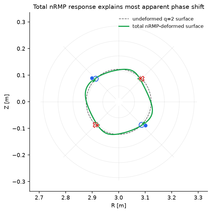
この解析平衡のヘリカルリップルは、(m,n)=(2,1) 磁気島を開く共鳴 RMP 成分ではありません。それでも近傍磁束面の幾何を変化させます。Newton 固定点を未変形の円形面と比較すると、その滑らかな変位が人工的な位相誤差として現れます。
ここではヘリカルリップルが磁力線 ODE に与える寄与
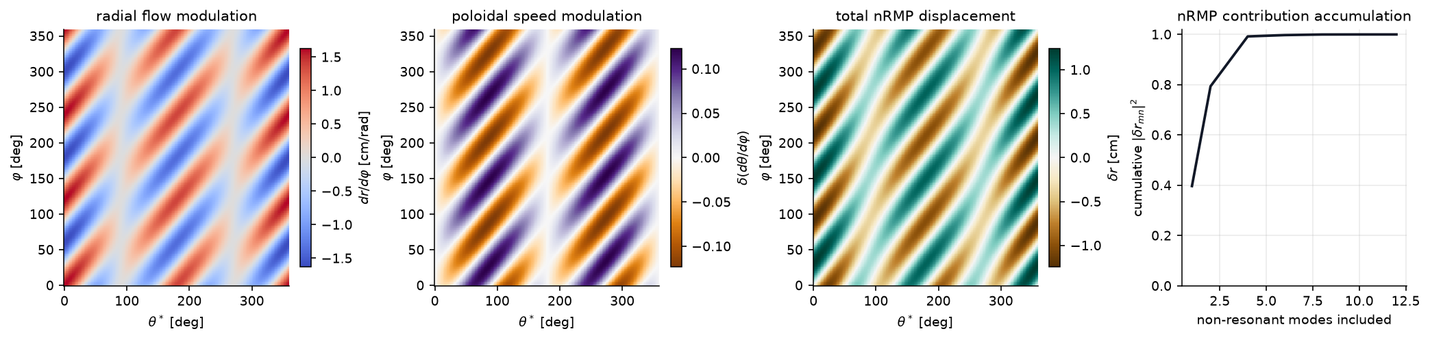
をサンプリングし、F_r と F_theta を Fourier 変換して、すべての非共鳴係数について非共鳴ホモロジカル方程式を解きます。応答オブジェクトは全変形と寄与ランキングを保持します。ランキングは診断であり、以下で使う変形は完全に和を取った nRMP 応答です。
[9]:
def helical_ripple_delta_B(eq_case):
    """Return the analytic helical-ripple contribution used by simple_stellarator."""
    def delta_B_helical(R, Z, phi):
        R_arr = np.asarray(R, dtype=float)
        Z_arr = np.asarray(Z, dtype=float)
        phi_arr = np.asarray(phi, dtype=float)
        theta = np.arctan2(Z_arr, R_arr - eq_case.R0)
        psi = eq_case.psi_ax(R_arr, Z_arr)
        dBR = eq_case.epsilon_h * eq_case.B0 * psi * np.cos(eq_case.m_h * theta - eq_case.n_h * phi_arr)
        return np.array([
            dBR,
            np.zeros_like(dBR, dtype=float),
            np.zeros_like(dBR, dtype=float),
        ])
    return delta_B_helical


def helical_velocity_response(eq_case, psi_res, n_theta=256, n_phi=256, include_shear=False):
    velocity = fieldline_velocity_spectrum_on_circular_surface(
        eq_case,
        helical_ripple_delta_B(eq_case),
        psi_res,
        n_theta=n_theta,
        n_phi=n_phi,
        m_max=8,
        n_max=8,
        min_amplitude=1e-12,
    )
    return velocity.nonresonant_response(include_shear=include_shear)


def helical_velocity_deformation(eq_case, psi_res, n_theta=256, n_phi=256, include_shear=False):
    response = helical_velocity_response(
        eq_case,
        psi_res,
        n_theta=n_theta,
        n_phi=n_phi,
        include_shear=include_shear,
    )
    return response.deformation, response.velocity.r_minor, response.velocity


case_label = 'RMP + analytic helical ripple'
if components and case_label in cyna_rows_by_case:
    rows = cyna_rows_by_case[case_label]
    eq_case = cyna_eq_by_case[case_label]
    response_helical = helical_velocity_response(eq_case, components[0].psi_res)
    deformation = response_helical.deformation
    velocity_helical = response_helical.velocity
    r_res = velocity_helical.r_minor
    projected_rows = project_fixed_points_to_deformed_surface(
        rows,
        eq_case,
        deformation,
        r_minor=r_res,
        theta_window=0.35,
    )

    print(
        'nRMP total response uses '
        f'{response_helical.n_nonresonant_modes} non-resonant modes '
        f'and excludes {response_helical.n_resonant_modes} resonant modes.'
    )
    print('Largest nRMP response contributors; these rank the sum but do not replace it:')
    print('{:>8} {:>12} {:>14} {:>14}'.format('(m,n)', 'detuning', '|delta_r_mn| cm', 'cum frac'))
    for contrib in response_helical.contribution_rows(top=6):
        print('({:>2d},{:>2d}) {:>12.3e} {:>14.4f} {:>14.3f}'.format(
            contrib.m,
            contrib.n,
            contrib.detuning,
            100.0 * contrib.radial_response_weight,
            contrib.cumulative_fraction,
        ))
    print()

    raw_max = max(abs(row.theta_error_deg) for row in rows)
    corrected_max = max(abs(row.theta_error_deg) for row in projected_rows)
    nearest_max = max(row.distance_cm for row in projected_rows)
    print(f'Raw circular-surface max |dtheta|:       {raw_max:.4f} deg')
    print(f'Deformed-surface-coordinate max |dtheta|: {corrected_max:.4f} deg')
    print(f'Max Newton-to-deformed-section distance:  {nearest_max:.3f} cm')
    print()
    header = '{:<4} {:>6} {:>12} {:>16} {:>13}'.format(
        'kind', 'branch', 'raw dtheta', 'deformed dtheta', 'distance [cm]'
    )
    print(header)
    print('-' * len(header))
    for row, proj in zip(rows, projected_rows):
        print('{:<4} {:>6d} {:>12.4f} {:>16.4f} {:>13.3f}'.format(
            row.predicted_kind,
            row.branch,
            row.theta_error_deg,
            proj.theta_error_deg,
            proj.distance_cm,
        ))

    theta_line = np.linspace(0.0, 2*np.pi, 721)
    R_circ = eq_case.R0 + r_res*np.cos(theta_line)
    Z_circ = r_res*np.sin(theta_line)
    R_def, Z_def = deformed_circular_section_rz(eq_case, r_res, deformation, theta_line)

    fig_def, ax_def = plt.subplots(figsize=(5.2, 4.8), constrained_layout=True)
    draw_pest_grid(ax_def, eq_case, alpha=0.16)
    ax_def.plot(R_circ, Z_circ, color='0.35', lw=0.9, ls='--', label='undeformed q=2 surface')
    ax_def.plot(R_def, Z_def, color='#16a34a', lw=1.8, label='total nRMP-deformed surface')

    for row, proj in zip(rows, projected_rows):
        color = '#2563eb' if row.predicted_kind == 'O' else '#dc2626'
        marker = 'o' if row.predicted_kind == 'O' else 'X'
        ax_def.plot([row.predicted_R, row.newton_R], [row.predicted_Z, row.newton_Z],
                    color=color, lw=0.8, alpha=0.35)
        ax_def.plot([proj.closest_R, row.newton_R], [proj.closest_Z, row.newton_Z],
                    color=color, lw=1.1, ls=':', alpha=0.9)
        ax_def.scatter(row.predicted_R, row.predicted_Z, marker=marker, s=72,
                       facecolors='none', edgecolors=color, linewidths=1.2, zorder=5)
        ax_def.scatter(proj.closest_R, proj.closest_Z, marker='D', s=42,
                       color='#16a34a', edgecolors='white', linewidths=0.45, zorder=6)
        ax_def.scatter(row.newton_R, row.newton_Z, marker=marker, s=44,
                       color=color, edgecolors='white', linewidths=0.5, zorder=7)

    lim = 1.12 * eq_case.r0
    ax_def.set_xlim(eq_case.R0 - lim, eq_case.R0 + lim)
    ax_def.set_ylim(-lim, lim)
    ax_def.set_aspect('equal')
    ax_def.set_xlabel('R [m]')
    ax_def.set_ylabel('Z [m]')
    ax_def.set_title('Total nRMP response explains most apparent phase shift')
    ax_def.legend(frameon=False, loc='upper right', fontsize=8)
    plt.show()

    TT_h, PP_h, dr_h, dtheta_h = response_helical.real_fields()
    counts_h, cumulative_h = response_helical.cumulative_contribution()
    theta_deg_h = np.degrees(velocity_helical.theta)
    phi_deg_h = np.degrees(velocity_helical.phi)
    fig_flow, axes_flow = plt.subplots(1, 4, figsize=(13.8, 3.2), constrained_layout=True)
    panels = [
        (velocity_helical.radial_velocity * 100.0, r'$dr/d\varphi$ [cm/rad]', 'radial flow modulation', 'coolwarm'),
        (velocity_helical.poloidal_velocity, r'$\delta(d\theta/d\varphi)$', 'poloidal speed modulation', 'PuOr'),
        (dr_h * 100.0, r'$\delta r$ [cm]', 'total nRMP displacement', 'BrBG'),
    ]
    for ax, (data, cbar_label, title, cmap) in zip(axes_flow[:3], panels):
        vmax = np.nanmax(np.abs(data))
        im = ax.pcolormesh(
            theta_deg_h,
            phi_deg_h,
            data,
            shading='auto',
            cmap=cmap,
            vmin=-vmax,
            vmax=vmax,
        )
        ax.set_xlabel(r'$\theta^*$ [deg]')
        ax.set_ylabel(r'$\varphi$ [deg]')
        ax.set_title(title)
        fig_flow.colorbar(im, ax=ax, label=cbar_label, shrink=0.85)
    axes_flow[3].plot(counts_h, cumulative_h, color='#111827', lw=1.8)
    axes_flow[3].set_ylim(0, 1.02)
    axes_flow[3].set_xlabel('non-resonant modes included')
    axes_flow[3].set_ylabel(r'cumulative $|\delta r_{mn}|^2$')
    axes_flow[3].set_title('nRMP contribution accumulation')
    axes_flow[3].grid(True, alpha=0.25)
    plt.show()
else:
    print('Non-resonant deformation check skipped because cyna rows are unavailable.')
nRMP total response uses 12 non-resonant modes and excludes 2 resonant modes.
Largest nRMP response contributors; these rank the sum but do not replace it:
   (m,n)     detuning |delta_r_mn| cm       cum frac
(-4, 3)    1.000e+00         0.3755          0.397
( 4,-3)   -1.000e+00         0.3755          0.794
(-2, 3)    2.000e+00         0.1877          0.893
( 2,-3)   -2.000e+00         0.1877          0.992
(-5, 3)    5.000e-01         0.0306          0.995
( 5,-3)   -5.000e-01         0.0306          0.997

Raw circular-surface max |dtheta|:       3.5877 deg
Deformed-surface-coordinate max |dtheta|: 1.4748 deg
Max Newton-to-deformed-section distance:  0.822 cm

kind branch   raw dtheta  deformed dtheta distance [cm]
-------------------------------------------------------
O         0       3.5877           0.6159         0.822
O         1       3.4195           0.7933         0.783
X         0       2.0428          -1.4748         0.250
X         1       1.9400          -1.1567         0.196
[MIXED_SPECTRUM] 1 つの面での混合 RMP/nRMP ワークフロー#
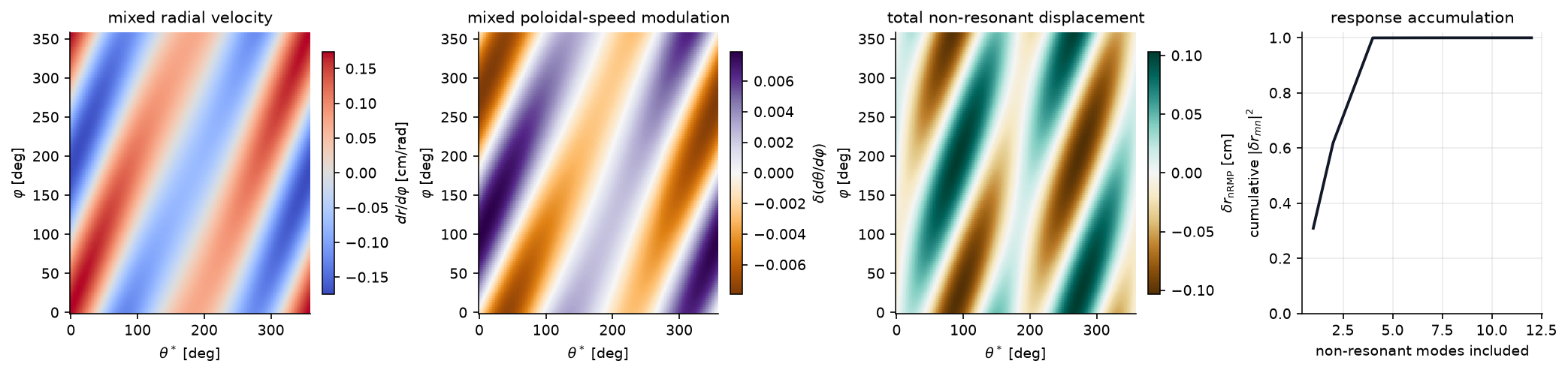
実際の摂動が 1 つのきれいな高調波だけを含むことはまれです。この例では、共鳴 (2,1) RMP と、m=1 項を含む 2 つの非共鳴成分を重ねます。モード表はサンプリングされた速度スペクトルを分類しますが、これは診断にすぎません。計算の nRMP 部分は全応答オブジェクトであり、滑らかな変位と速度変調を描く前に、すべての非共鳴行を和に含めます。
[10]:
mixed_delta_B = compose_magnetic_perturbations(
    delta_B_RMP,
    radial_rmp_field_template(3, 1, amplitude=2.0e-4, phase=0.20, axis_R=eq.R0),
    radial_rmp_field_template(1, 1, amplitude=1.5e-4, phase=0.40, axis_R=eq.R0),
)

mixed_velocity = fieldline_velocity_spectrum_on_circular_surface(
    eq,
    mixed_delta_B,
    psi_res_21,
    n_theta=160,
    n_phi=128,
    m_max=5,
    n_max=4,
    min_amplitude=1e-13,
)
mixed_rows = rmp_nrmp_mode_rows(
    mixed_velocity.radial_spectrum,
    mixed_velocity.iota,
    resonance_tol=1e-10,
    top=12,
    min_amplitude=1e-8,
)
mixed_response = mixed_velocity.nonresonant_response(include_shear=True, resonance_tol=1e-10)

print(f'Local iota on q=2 surface: {mixed_velocity.iota:.6f}')
print(
    'Total nRMP response uses '
    f'{mixed_response.n_nonresonant_modes} non-resonant modes; '
    f'{mixed_response.n_resonant_modes} resonant modes are left for island analysis.'
)
print()
print('RMP/nRMP mode classification diagnostic:')
print('{:<5} {:>8} {:>12} {:>12} {:>12}'.format('kind', '(m,n)', 'detuning', '|F_r mn|', 'phase [deg]'))
print('-' * 56)
for row in mixed_rows:
    print('{:<5} ({:>2d},{:>2d}) {:>12.3e} {:>12.3e} {:>12.2f}'.format(
        row.kind,
        row.m,
        row.n,
        row.detuning,
        row.amplitude,
        row.phase_deg,
    ))

print()
print('Largest contributors to the total nRMP radial response:')
print('{:>8} {:>12} {:>14} {:>14}'.format('(m,n)', 'detuning', '|delta_r_mn| cm', 'cum frac'))
for contrib in mixed_response.contribution_rows(top=8):
    print('({:>2d},{:>2d}) {:>12.3e} {:>14.4f} {:>14.3f}'.format(
        contrib.m,
        contrib.n,
        contrib.detuning,
        100.0 * contrib.radial_response_weight,
        contrib.cumulative_fraction,
    ))

mixed_deformation = mixed_response.deformation
TT_mix, PP_mix, nonres_dr_mix, nonres_dtheta_mix = mixed_response.real_fields()
counts_mix, cumulative_mix = mixed_response.cumulative_contribution()

theta_deg_mix = np.degrees(mixed_velocity.theta)
phi_deg_mix = np.degrees(mixed_velocity.phi)
fig_mix, axes_mix = plt.subplots(1, 4, figsize=(13.8, 3.2), constrained_layout=True)
panels = [
    (mixed_velocity.radial_velocity * 100.0, r'$dr/d\varphi$ [cm/rad]', 'mixed radial velocity', 'coolwarm'),
    (mixed_velocity.poloidal_velocity, r'$\delta(d\theta/d\varphi)$', 'mixed poloidal-speed modulation', 'PuOr'),
    (nonres_dr_mix * 100.0, r'$\delta r_\mathrm{nRMP}$ [cm]', 'total non-resonant displacement', 'BrBG'),
]
for ax, (data, label, title, cmap) in zip(axes_mix[:3], panels):
    vmax = np.nanmax(np.abs(data))
    im = ax.pcolormesh(
        theta_deg_mix,
        phi_deg_mix,
        data,
        shading='auto',
        cmap=cmap,
        vmin=-vmax,
        vmax=vmax,
    )
    ax.set_xlabel(r'$\theta^*$ [deg]')
    ax.set_ylabel(r'$\varphi$ [deg]')
    ax.set_title(title)
    fig_mix.colorbar(im, ax=ax, label=label, shrink=0.86)
axes_mix[3].plot(counts_mix, cumulative_mix, color='#111827', lw=1.8)
axes_mix[3].set_ylim(0, 1.02)
axes_mix[3].set_xlabel('non-resonant modes included')
axes_mix[3].set_ylabel(r'cumulative $|\delta r_{mn}|^2$')
axes_mix[3].set_title('response accumulation')
axes_mix[3].grid(True, alpha=0.25)
plt.show()
Local iota on q=2 surface: 0.500000
Total nRMP response uses 12 non-resonant modes; 2 resonant modes are left for island analysis.

RMP/nRMP mode classification diagnostic:
kind     (m,n)     detuning     |F_r mn|  phase [deg]
--------------------------------------------------------
RMP   (-2, 1)    0.000e+00    6.087e-04        -0.23
RMP   ( 2,-1)    0.000e+00    6.087e-04         0.23
nRMP  (-3, 1)   -5.000e-01    1.442e-04        -9.53
nRMP  ( 3,-1)    5.000e-01    1.442e-04         9.53
nRMP  (-1, 1)    5.000e-01    1.131e-04       -18.07
nRMP  ( 1,-1)   -5.000e-01    1.131e-04        18.07
nRMP  ( 4,-1)    1.000e+00    5.144e-06        10.91
nRMP  (-4, 1)   -1.000e+00    5.144e-06       -10.91
nRMP  ( 0,-1)   -1.000e+00    3.906e-06        21.49
nRMP  ( 0, 1)    1.000e+00    3.906e-06       -21.49
nRMP  (-5, 1)   -1.500e+00    5.000e-08       -11.46
nRMP  ( 5,-1)    1.500e+00    5.000e-08        11.46

Largest contributors to the total nRMP radial response:
   (m,n)     detuning |delta_r_mn| cm       cum frac
(-3, 1)   -5.000e-01         0.0288          0.310
( 3,-1)    5.000e-01         0.0288          0.619
(-1, 1)    5.000e-01         0.0226          0.809
( 1,-1)   -5.000e-01         0.0226          1.000
( 4,-1)    1.000e+00         0.0005          1.000
(-4, 1)   -1.000e+00         0.0005          1.000
( 0, 1)    1.000e+00         0.0004          1.000
( 0,-1)   -1.000e+00         0.0004          1.000
[ORDER_ANALYSIS] 摂動次数の確認#
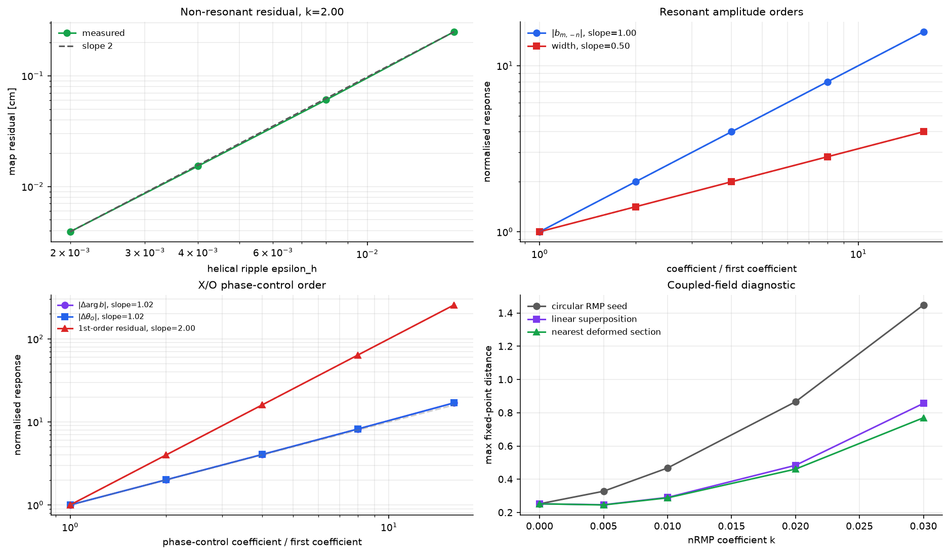
再利用可能なワークフローは、いくつかの小さなヘルパーにまとまりました。 scan_nonresonant_residual_order, scan_rmp_amplitude_order, scan_rmp_phase_order, scan_rmp_resolution_convergence、および plot_perturbation_order_summary。
Fourier 規約が固定されると、期待される次数は単純です。
nRMP 面形状残差:一次変形は
O(k^2)の写像残差を残すはずです。RMP 共鳴係数:
delta B = k fでは Fourier 線形性により|b_{m,-n}| ~ kです。島幅:Rutherford/Nardon 振り子幅は
w ~ sqrt(|b_{m,-n}|)とスケールするため、w ~ k^{1/2}です。X/O 位相:位相は振幅ではなく
arg(b_{m,-n})に制御されます。厳密な関係はm*Delta theta_O + Delta arg(b_{m,-n}) = 0です。
位相制御の次数には発散なしテンプレート radial_rmp_field_template を使います。この位相パラメータは、重要な m=1 ケースを含めて div(delta B)=0 を保ったまま共鳴係数位相を変えます。意図的にやや非線形な制御位相 alpha(k)=k+eta*k^2 をテストします。そのため一次の生の k 則に対する残差は O(k^2) とスケールするはずです。
[11]:
def component_for_rmp_template(amplitude=1.0e-3, phase=0.0, n_theta=128, n_phi=64):
    return find_resonant_components_analytic(
        eq,
        radial_rmp_field_template(base_m, base_n, amplitude=amplitude, phase=phase, axis_R=eq.R0),
        base_m=base_m,
        base_n=base_n,
        max_harmonic=1,
        n_theta=n_theta,
        n_phi=n_phi,
        min_amplitude=1e-16,
        verbose=False,
    )[0]


def deformed_torus_map_residual(epsilon_h, n_alpha=12):
    eq_case = simple_stellarator(
        R0=eq.R0, r0=eq.r0, B0=eq.B0,
        q0=eq.q0, q1=eq.q1,
        m_h=eq.m_h, n_h=eq.n_h, epsilon_h=float(epsilon_h),
    )
    psi_res = eq_case.resonant_psi(base_m, base_n)[0]
    deformation, r_res, _ = helical_velocity_deformation(
        eq_case, psi_res, n_theta=128, n_phi=128, include_shear=True
    )
    iota = 1.0 / float(eq_case.q_of_psi(psi_res))

    def surface(alpha, phi):
        alpha_arr = np.asarray(alpha)
        return (
            r_res + deformation.section_r(alpha_arr, phi),
            alpha_arr + deformation.section_theta(alpha_arr, phi),
        )

    def rhs(phi, state):
        radius, theta = state
        R = eq_case.R0 + radius*np.cos(theta)
        psi_here = (radius / eq_case.r0)**2
        q_here = float(eq_case.q_of_psi(psi_here))
        Bphi = eq_case.B0 * eq_case.R0 / R
        delta_BR = eq_case.epsilon_h * eq_case.B0 * psi_here * np.cos(eq_case.m_h * theta - eq_case.n_h * phi)
        return [
            R * delta_BR * np.cos(theta) / Bphi,
            1.0/q_here - R * delta_BR * np.sin(theta) / (radius * Bphi),
        ]

    residual = deformed_surface_map_residual(
        surface,
        rhs,
        iota,
        alpha_values=np.linspace(0.0, 2*np.pi, n_alpha, endpoint=False),
        state_to_cartesian=lambda state, phi: [
            eq_case.R0 + float(state[0])*np.cos(float(state[1])),
            float(state[0])*np.sin(float(state[1])),
        ],
    )
    return residual.max_residual


def max_helical_deformation_cm(n_theta, n_phi):
    velocity = fieldline_velocity_spectrum_on_circular_surface(
        eq,
        helical_ripple_delta_B(eq),
        psi_res_21,
        n_theta=max(64, n_theta),
        n_phi=max(64, n_phi),
        m_max=8,
        n_max=8,
        min_amplitude=1e-12,
    )
    deformation = velocity.nonresonant_deformation(include_shear=True)
    TT, PP = np.meshgrid(velocity.theta, velocity.phi, indexing='xy')
    return 100.0 * float(np.nanmax(np.abs(deformation.real_field_r(TT, PP))))


nonres_eps = np.array([0.002, 0.004, 0.008, 0.016])
rmp_k = np.array([2.5e-4, 5e-4, 1e-3, 2e-3, 4e-3])
phase_controls = np.array([0.01, 0.02, 0.04, 0.08, 0.16])
phase_eta = 0.4

nonres_scan = scan_nonresonant_residual_order(nonres_eps, deformed_torus_map_residual)
rmp_amp_scan = scan_rmp_amplitude_order(
    rmp_k,
    lambda k: component_for_rmp_template(amplitude=k, phase=0.0, n_theta=64, n_phi=32),
)
phase_base = component_for_rmp_template(amplitude=1e-3, phase=0.0, n_theta=128, n_phi=64)
phase_scan = scan_rmp_phase_order(
    phase_controls,
    lambda k: component_for_rmp_template(
        amplitude=1e-3,
        phase=float(k) + phase_eta*float(k)*float(k),
        n_theta=128,
        n_phi=64,
    ),
    base_component=phase_base,
)
resolution_scan = scan_rmp_resolution_convergence(
    [(32, 16), (64, 32), (128, 64), (256, 128)],
    lambda n_theta, n_phi: component_for_rmp_template(
        amplitude=1e-3, phase=0.0, n_theta=n_theta, n_phi=n_phi
    ),
    deformation_metric_factory=max_helical_deformation_cm,
)

comp_pos = component_for_rmp_template(amplitude=1e-3, phase=0.0, n_theta=64, n_phi=32)
comp_neg = component_for_rmp_template(amplitude=-1e-3, phase=0.0, n_theta=64, n_phi=32)
sign_phase_jump_deg = float(np.degrees(np.angle(comp_neg.b_mn / comp_pos.b_mn)))

print(f'Non-resonant deformation residual slope = {nonres_scan.slope:.3f} (expected 2)')
print(f'Positive RMP: |b_mn| slope =             {rmp_amp_scan.b_fit.slope:.3f} (expected 1)')
print(f'Positive RMP: island half-width slope =  {rmp_amp_scan.width_fit.slope:.3f} (expected 0.5)')
print(f'Positive RMP: X/O phase span:           {rmp_amp_scan.phase_span_deg:.3e} deg')
print(f'Negative coefficient: arg jump:         {sign_phase_jump_deg:.1f} deg')
print(f'  +k: O={np.degrees(comp_pos.opoint_theta):.1f} deg, X={np.degrees(comp_pos.xpoint_theta):.1f} deg')
print(f'  -k: O={np.degrees(comp_neg.opoint_theta):.1f} deg, X={np.degrees(comp_neg.xpoint_theta):.1f} deg')
print(f'Phase template: |Delta arg b| slope =    {phase_scan.b_phase_fit.slope:.3f} (locally expected 1)')
print(f'Phase template: |Delta theta_O| vs |Delta arg b| slope = {phase_scan.opoint_vs_b_phase_fit.slope:.3f} (expected 1)')
print(f'Phase template: max |m Delta theta_O + Delta arg b|: {phase_scan.max_exact_relation_residual:.3e} rad')
print(f'Phase template: first-order residual slope = {phase_scan.first_order_residual_fit.slope:.3f} (expected 2)')

print()
print('Resolution convergence against the finest RMP spectrum grid:')
print('{:>8} {:>6} {:>12} {:>14} {:>14} {:>14}'.format(
    'n_theta', 'n_phi', 'rel |b| err', 'phase err deg', 'rel width err', 'max |dr| cm'
))
for row in resolution_scan.rows:
    print(f'{row.n_theta:8d} {row.n_phi:6d} {row.relative_b_error:12.3e} '
          f'{row.phase_error_deg:14.3e} {row.relative_width_error:14.3e} '
          f'{row.deformation_metric:14.4f}')

coupling_sweep = None
if components:
    component = components[0]

    def coupled_distances(eps_h):
        eq_case = simple_stellarator(
            R0=eq.R0, r0=eq.r0, B0=eq.B0,
            q0=eq.q0, q1=eq.q1,
            m_h=eq.m_h, n_h=eq.n_h, epsilon_h=float(eps_h),
        )
        rows = compare_cyna_fixed_points_for_component(
            sample_stellarator_cylindrical_field(
                eq_case, delta_B_RMP, nR=128, nPhi=128, label=f'coupled_rmp_eps_{eps_h:.3f}',
            ),
            component,
            eq_case,
            DPhi=0.015,
            max_iter=80,
            tol=1e-11,
            n_threads=4,
        )
        raw_cm = max(np.hypot(row.newton_R - row.predicted_R, row.newton_Z - row.predicted_Z) for row in rows) * 100.0
        if eps_h == 0.0:
            return raw_cm, raw_cm, raw_cm
        deformation, r_res, _ = helical_velocity_deformation(eq_case, component.psi_res, include_shear=True)
        superposed_cm = max(
            np.hypot(
                float(deformed_circular_section_rz(eq_case, r_res, deformation, row.predicted_theta)[0]) - row.newton_R,
                float(deformed_circular_section_rz(eq_case, r_res, deformation, row.predicted_theta)[1]) - row.newton_Z,
            ) for row in rows
        ) * 100.0
        projected = project_fixed_points_to_deformed_surface(rows, eq_case, deformation, r_minor=r_res)
        return raw_cm, superposed_cm, max(row.distance_cm for row in projected)

    try:
        coupling_sweep = scan_coupled_fixed_point_sweep(np.array([0.0, 0.005, 0.01, 0.02, 0.03]), coupled_distances)
    except ImportError as exc:
        print('Coupled cyna sweep skipped:', exc)

if coupling_sweep is not None:
    print()
    print('Coupled RMP + helical ripple, fixed RMP amplitude:')
    print('{:>9} {:>12} {:>16} {:>16}'.format('epsilon_h', 'raw [cm]', 'superposed [cm]', 'nearest [cm]'))
    for eps_h, raw_cm, superposed_cm, nearest_cm in zip(
        coupling_sweep.k, coupling_sweep.raw_distance,
        coupling_sweep.superposed_distance, coupling_sweep.nearest_deformed_distance,
    ):
        print(f'{eps_h:9.3f} {raw_cm:12.4f} {superposed_cm:16.4f} {nearest_cm:16.4f}')

fig_order, axes_order = plot_perturbation_order_summary(
    nonresonant=nonres_scan,
    rmp_amplitude=rmp_amp_scan,
    rmp_phase=phase_scan,
    coupling=coupling_sweep,
    residual_scale=100.0,
    residual_label='map residual [cm]',
    coefficient_label='helical ripple epsilon_h',
)
plt.show()
Non-resonant deformation residual slope = 1.999 (expected 2)
Positive RMP: |b_mn| slope =             1.000 (expected 1)
Positive RMP: island half-width slope =  0.500 (expected 0.5)
Positive RMP: X/O phase span:           0.000e+00 deg
Negative coefficient: arg jump:         180.0 deg
  +k: O=135.0 deg, X=45.0 deg
  -k: O=45.0 deg, X=135.0 deg
Phase template: |Delta arg b| slope =    1.020 (locally expected 1)
Phase template: |Delta theta_O| vs |Delta arg b| slope = 1.000 (expected 1)
Phase template: max |m Delta theta_O + Delta arg b|: 4.441e-16 rad
Phase template: first-order residual slope = 2.000 (expected 2)

Resolution convergence against the finest RMP spectrum grid:
 n_theta  n_phi  rel |b| err  phase err deg  rel width err    max |dr| cm
      32     16    0.000e+00      0.000e+00      0.000e+00         1.2408
      64     32    0.000e+00      0.000e+00      0.000e+00         1.2408
     128     64    0.000e+00      0.000e+00      0.000e+00         1.2408
     256    128    0.000e+00      0.000e+00      0.000e+00         1.2408

Coupled RMP + helical ripple, fixed RMP amplitude:
epsilon_h     raw [cm]  superposed [cm]     nearest [cm]
    0.000       0.2524           0.2524           0.2524
    0.005       0.3280           0.2467           0.2455
    0.010       0.4678           0.2908           0.2883
    0.020       0.8661           0.4838           0.4610
    0.030       1.4484           0.8564           0.7698
[ISLAND_WIDTHS] 島幅棒グラフと Chirikov オーバーラップ図#
Chirikov オーバーラップパラメータ は
で定義されます。ここで \(w_i\) は半幅、\(r_i\) は隣接する磁気島の径方向位置です。\(\sigma \gtrsim 1\) になると確率的輸送が始まります。
[12]:
fig_iw, (ax_bar, ax_q) = plt.subplots(1, 2, figsize=(9, 3.8))

# ── (a) Island width bar chart ───────────────────────────────────────────
labels = [f'$({c.m},{c.n})$\nq={c.q_res:.2f}' for c in components]
widths_cm = [c.half_width_r * 100 for c in components]
colors_bar = [ISLAND_CMAPS[(c.harmonic_order - 1) % len(ISLAND_CMAPS)] for c in components]

x_pos = np.arange(len(components))
bars = ax_bar.bar(x_pos, widths_cm, color=colors_bar, edgecolor='k',
                  linewidth=0.7, alpha=0.85, width=0.55)
for bar, w in zip(bars, widths_cm):
    ax_bar.text(bar.get_x() + bar.get_width()/2, w + 0.05,
                f'{w:.2f}', ha='center', va='bottom', fontsize=8)

ax_bar.set_xticks(x_pos)
ax_bar.set_xticklabels(labels, fontsize=8)
ax_bar.set_ylabel('Island half-width (cm)')
ax_bar.set_title('Island Width by Harmonic')
ax_bar.set_ylim(0, max(widths_cm)*1.25 if widths_cm else 1)

# ── (b) q-profile with island width bands ───────────────────────────────
psi_arr = np.linspace(0, 1, 200)
r_arr = np.sqrt(psi_arr) * eq.r0
q_arr = eq.q_of_psi(psi_arr)

ax_q.plot(r_arr * 100, q_arr, 'k-', linewidth=1.5, label='q(r)')
ax_q.set_xlabel('r (cm)')
ax_q.set_ylabel('Safety factor q')
ax_q.set_title('q-profile with Island Width Bands')

# Draw horizontal bands for each resonance
chirikov_pairs = []
for c in components:
    color = ISLAND_CMAPS[(c.harmonic_order - 1) % len(ISLAND_CMAPS)]
    r_res = np.sqrt(c.psi_res) * eq.r0 * 100  # cm
    w_r = c.half_width_r * 100  # cm
    q_res = c.q_res
    # Island band in r
    ax_q.axvspan(r_res - w_r, r_res + w_r, alpha=0.25, color=color, zorder=2)
    ax_q.axhline(q_res, color=color, lw=0.8, linestyle='--', alpha=0.7)
    ax_q.text(r_res + w_r + 0.2, q_res, f'$({c.m},{c.n})$',
              color=color, fontsize=8, va='center')
    chirikov_pairs.append((r_res, w_r))

# Chirikov overlap
if len(chirikov_pairs) >= 2:
    for i in range(len(chirikov_pairs) - 1):
        r1, w1 = chirikov_pairs[i]
        r2, w2 = chirikov_pairs[i+1]
        gap = abs(r2 - r1)
        sigma = (w1 + w2) / gap if gap > 0 else float('inf')
        print(f'Chirikov sigma between ({components[i].m},{components[i].n}) and ({components[i+1].m},{components[i+1].n}): {sigma:.3f}')

ax_q.set_xlim(0, eq.r0 * 100 * 1.05)
ax_q.grid(True, alpha=0.3)

plt.tight_layout()
plt.show()
[MN_SPECTRUM] 2 次元 Fourier スペクトルヒートマップ#
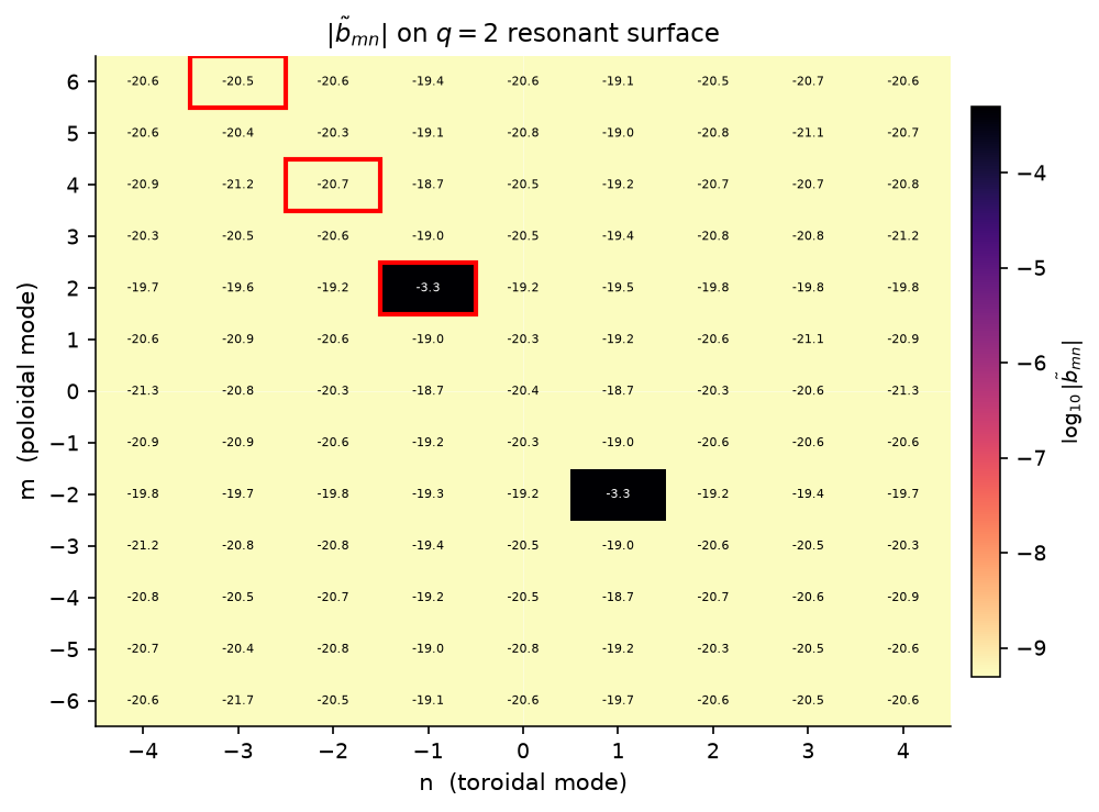
主共鳴面上で発散なし RMP テンプレートの完全な \((m,n)\) Fourier スペクトルを計算します。共鳴モード \((2,-1)\) と、それに駆動される高調波を強調表示します。上の混合スペクトル節は、共鳴行と非共鳴行を離調で分類する補助ビューです。
[13]:
psi_res_21 = eq.resonant_psi(2, 1)[0]
print(f'Computing (m,n) spectrum on q=2 surface (psi={psi_res_21:.3f}), n_theta=48, n_phi=48...')
b_mn = compute_mn_spectrum(
    delta_B_RMP,
    S=psi_res_21,
    equilibrium=eq,
    m_max=6,
    n_max=4,
    n_theta=48,
    n_phi=48,
)
print(f'Spectrum shape: {b_mn.shape}')

fig_sp, ax_sp = plt.subplots(figsize=(7, 5))
plot_mn_heatmap(
    b_mn, m_max=6, n_max=4,
    ax=ax_sp,
    log_scale=True,
    title=r'$|\tilde{b}_{mn}|$ on $q=2$ resonant surface',
    cmap='magma_r',
    highlight_modes=[(2, -1), (4, -2), (6, -3)],
)
plt.tight_layout()
plt.show()
Computing (m,n) spectrum on q=2 surface (psi=0.167), n_theta=48, n_phi=48...
Spectrum shape: (13, 9)
[MAGNETIC_SPECTRUM_ATLAS] 多成分 \(B^r\) スペクトルアトラス#
上の単一面ヒートマップは支配的な RMP 行の確認には有用ですが、本番の磁気トポロジー解析では通常ファミリービューが必要です。ここでは発散なしの多成分摂動を構築し、Nardon 方式の反変径方向スペクトル \(\tilde b^1_{mn}=\delta B^1/B_0^3\) を径方向スタック上で計算し、要求された共鳴行をまとめて解析します。
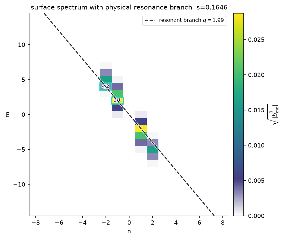
下のユーティリティは意図的にモジュール化してあります。表示するアトラスは、より広い符号付き Fourier 窓、97 個の径方向面、amplitude_scale='sqrt'、ゼロ/欠損行用の白マスクを使います。非対数カラーマップは同じ白の基準から始まるため、ほぼゼロの係数がマスクされた背景から人工的に分離して見えることを避けられます。符号付き軸は計算されたスペクトル内の実際の Fourier 行を示します。実場では (m,n) は (-m,-n) と共役ですが、(m,n) と (m,-n)
は摂動モデルが追加の対称性を課さない限り、独立した反対ヘリシティ行です。amplitude_scale='log10' は、目的が視覚的パターン認識ではなく厳密なダイナミックレンジ監査である場合には引き続き有用です。
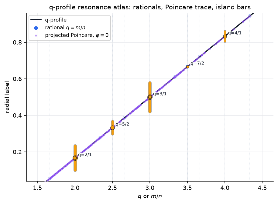
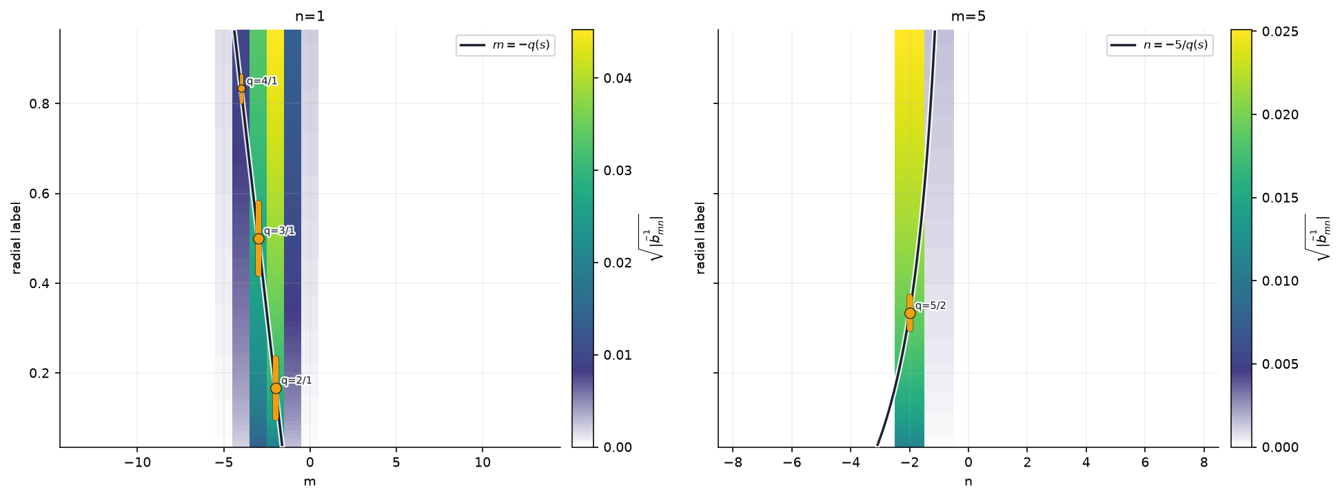
plot_rational_surface_mapは、任意の q プロファイル、低次有理面マーカー、投影 Poincaré 点、島幅バーを(m/n, s)平面に合成します。plot_spectrum_heatmap(..., renderer='pcolormesh')は推奨される面スペクトルビューです。反対ヘリシティ枝を描かず、物理的な共鳴分枝m=-q n_Fを重ね描きできます。plot_spectrum_bar3dは、支配的な行を回転、ズーム、ホバー確認できる対話的な Plotly 図を返します。plot_radial_mode_heatmap(fixed_n=..., resonant_sign=+1)は固定 Fourier \(n\) で全 \(m\) 行を追跡し、負の \(m\) 半平面に正の q 分枝 \(m=-nq(s)\) を描きます。plot_radial_mode_heatmap(fixed_m=..., axis_convention='fourier')は実際の Fourier \(n\) 行を追跡し、正の q 分枝 \(n=-m/q(s)\) を描きます。q 曲線と島幅バーは独立に切り替えできます。
黄色の垂直バーは、低次有理面での単一係数 Nardon 半幅推定を示します。バーの太さは共鳴係数振幅に応じてスケールします。これらは任意の重ね描きであり、ヒートマップそのものの一部ではありません。各径方向マップには物理的に共鳴する曲線だけを描きます。反対ヘリシティ枝は共役診断ではないため、ここでは意図的に鏡映していません。複数の高調波が同じ既約有理面を共有する場合、真の有限振幅島幅は結合した共鳴ハミルトニアンから計算すべきです。行ごとのバーは診断であり、その非線形和としての幅ではありません。
[14]:
delta_B_multi_rmp = compose_magnetic_perturbations(
    radial_rmp_field_template(2, 1, amplitude=5.0e-4, phase=0.00, axis_R=eq.R0),
    radial_rmp_field_template(3, 1, amplitude=2.4e-4, phase=0.55, axis_R=eq.R0),
    radial_rmp_field_template(5, 2, amplitude=1.6e-4, phase=-0.35, axis_R=eq.R0),
)

S_scan = np.linspace(0.04, 0.96, 97)
theta_spec = np.linspace(0.0, 2*np.pi, 160, endpoint=False)
phi_spec = np.linspace(0.0, 2*np.pi, 96, endpoint=False)

theta_grid = theta_spec[None, None, :]
phi_grid = phi_spec[:, None, None]
r_scan = eq.r0 * np.sqrt(S_scan)[None, :, None]
R_stack = eq.R0 + r_scan * np.cos(theta_grid)
Z_stack = r_scan * np.sin(theta_grid)
R_stack = np.repeat(R_stack, phi_spec.size, axis=0)
Z_stack = np.repeat(Z_stack, phi_spec.size, axis=0)
Phi_stack = phi_grid + np.zeros_like(R_stack)

dBR_stack, dBZ_stack, dBphi_stack = delta_B_multi_rmp(R_stack, Z_stack, Phi_stack)
Bphi0_stack = eq.B0 * eq.R0 / np.maximum(R_stack, 1.0e-12)
tilde_b1_grid = nardon_radial_perturbation(
    R_stack,
    Z_stack,
    phi_spec,
    theta_spec,
    dBR_stack,
    dBZ_stack,
    dBphi_stack,
    S_scan,
    denominator_B_phi=Bphi0_stack,
)
magnetic_spectrum = radial_perturbation_Fourier_spectrum(
    tilde_b1_grid,
    theta_spec,
    phi_spec,
    radial_labels=S_scan,
    m_max=14,
    n_max=8,
    min_amplitude=1.0e-14,
)
q_scan = eq.q_of_psi(S_scan)
n_scan = [1, 2, 3]
m_scan = {1: range(1, 9), 2: range(2, 13), 3: range(3, 15)}
chains_multi = analyze_resonant_island_chains_multi_n(
    magnetic_spectrum,
    q_scan,
    n_values=n_scan,
    m_values=m_scan,
    min_b_res=1.0e-8,
)

print(f'Radial spectrum: {S_scan.size} surfaces, {magnetic_spectrum.m.size} retained Fourier rows over |m|<=14, |n|<=8.')
print(f'Multi-RMP analysis found {len(chains_multi)} resonant island-chain estimates.')
print('{:>7} {:>9} {:>9} {:>12} {:>12} {:>10}'.format('(m,n)', 's_res', 'q_res', 'b_res', 'half_width', 'phase'))
for chain in sorted(chains_multi, key=lambda item: item.b_res, reverse=True)[:8]:
    print('({:>2d},{:>1d}) {:>9.4f} {:>9.4f} {:>12.3e} {:>12.3e} {:>9.1f}°'.format(
        chain.m, chain.n, chain.radial_label, chain.q, chain.b_res, chain.half_width, np.degrees(chain.phase)
    ))

review_root = PROJECT_ROOT if PROJECT_ROOT is not None else pathlib.Path.cwd()
review_dir = review_root / 'pyna_output/magnetic_spectrum_review'
review_dir.mkdir(parents=True, exist_ok=True)

poincare_trace = None
if 'R_cross_p0' in globals() and len(R_cross_p0):
    S_p0 = np.clip(((R_cross_p0 - eq.R0)**2 + Z_cross_p0**2) / eq.r0**2, 0.0, 1.0)
    q_p0 = eq.q_of_psi(S_p0)
    poincare_trace = PoincareRationalTrace(
        ratio=q_p0,
        radial_label=S_p0,
        label=r'projected Poincare, $\varphi=0$',
    )

fig_qmap, ax_qmap, rational_markers = plot_rational_surface_map(
    S_scan,
    q_scan,
    n_values=n_scan,
    m_values=m_scan,
    chains=chains_multi,
    poincare=poincare_trace,
    show_poincare=poincare_trace is not None,
    max_island_bars=12,
    annotate_rationals=False,
    title='q-profile resonance atlas: rationals, Poincare trace, island bars',
)
fig_qmap.savefig(review_dir / '01_q_profile_resonance_map.png', dpi=180, bbox_inches='tight', facecolor='white')
plt.show()

surface_index = int(np.argmin(np.abs(S_scan - psi_res_21)))
surface_label = float(S_scan[surface_index])
chains_surface = [chain for chain in chains_multi if abs(chain.radial_label - surface_label) <= 0.08]
fig_surface, ax_surface = plt.subplots(figsize=(6.7, 5.7))
plot_spectrum_heatmap(
    magnetic_spectrum,
    radial_index=surface_index,
    m_values=np.arange(-14, 15),
    n_values=np.arange(-8, 9),
    chains=chains_surface,
    q_value=float(q_scan[surface_index]),
    renderer='pcolormesh',
    amplitude_scale='sqrt',
    mask_zeros=True,
    ax=ax_surface,
    cmap='viridis',
    title='surface spectrum with physical resonance branch',
)
fig_surface.savefig(review_dir / '02_surface_pcolormesh_atlas.png', dpi=180, bbox_inches='tight', facecolor='white')
plt.show()

fig_bar3d = plot_spectrum_bar3d(
    magnetic_spectrum,
    radial_index=surface_index,
    m_values=np.arange(-10, 11),
    n_values=np.arange(-6, 7),
    amplitude_scale='sqrt',
    range_mode='nonzero',
    bar_width=0.9,
    z_aspect=0.72,
    title='interactive 3D spectrum bars',
)
fig_bar3d.write_html(str(review_dir / '04_surface_plotly_bar3d.html'), include_plotlyjs='cdn')
try:
    fig_bar3d.write_image(str(review_dir / '04_surface_plotly_bar3d.png'), width=1040, height=650, scale=2)
except Exception as exc:
    print(f'Plotly static PNG export skipped: {exc}')
fig_bar3d.show()

fig_radial, axes_radial = plt.subplots(1, 2, figsize=(13.2, 4.9), sharey=True)
plot_radial_mode_heatmap(
    magnetic_spectrum,
    fixed_n=1,
    mode_values=np.arange(-14, 15),
    resonant_sign=1,
    q_profile=q_scan,
    chains=chains_multi,
    renderer='pcolormesh',
    amplitude_scale='sqrt',
    mask_zeros=True,
    ax=axes_radial[0],
    cmap='viridis',
    title='n=1',
)
plot_radial_mode_heatmap(
    magnetic_spectrum,
    fixed_m=5,
    mode_values=np.arange(-8, 9),
    axis_convention='fourier',
    q_profile=q_scan,
    chains=chains_multi,
    renderer='pcolormesh',
    amplitude_scale='sqrt',
    mask_zeros=True,
    ax=axes_radial[1],
    cmap='viridis',
    title='m=5',
)
plt.tight_layout()
fig_radial.savefig(review_dir / '03_radial_fixed_n_fixed_m_maps.png', dpi=180, bbox_inches='tight', facecolor='white')
plt.show()
Radial spectrum: 97 surfaces, 22 retained Fourier rows over |m|<=14, |n|<=8.
Multi-RMP analysis found 7 resonant island-chain estimates.
  (m,n)     s_res     q_res        b_res   half_width      phase
( 2,1)    0.1667    2.0000    1.661e-03    6.655e-02       0.6°
( 3,1)    0.5000    3.0000    1.535e-03    7.836e-02      27.6°
( 5,2)    0.3333    2.5000    7.401e-04    3.512e-02     -20.1°
( 4,1)    0.8333    4.0000    1.665e-04    2.980e-02      30.1°
( 6,2)    0.5000    3.0000    6.400e-05    1.131e-02     -20.1°
( 4,2)    0.1667    2.0000    2.132e-05    5.332e-03     -20.1°
( 7,2)    0.6667    3.5000    1.742e-06    2.016e-03     -20.1°
Data type cannot be displayed: application/vnd.plotly.v1+json
[PUBLICATION_FIGURE] 多 phi 6 パネル図#
同じ断面ヘルパーは、コンパクトな多断面レイアウトにもスケールします。O/X マーカー、O-point 島幅バー、局所安定枝はトロイダル角とともに回転し、PEST 風格子は各パネルで座標の意味を見える状態に保ちます。
[15]:
fig_pub, axes_pub = plot_rmp_resonance_sections(
    all_sections_data,
    phi_sections,
    eq=eq,
    components=components,
    colors=ISLAND_CMAPS,
    ncols=3,
    figsize=(12.0, 7.0),
    point_size=1.6,
    point_alpha=0.42,
    compact=True,
    overlays=('pest_grid', 'poincare', 'resonant_surfaces', 'stable_branches', 'island_width_bars', 'xo'),
    title=(
        'Stellarator RMP resonance: Poincare points, X/O geometry, '
        'island-width bars, stable branches, and PEST-style grid'
    ),
)

out_path = pathlib.Path('pyna_output/rmp_resonance_publication.png')
out_path.parent.mkdir(exist_ok=True)
fig_pub.savefig(str(out_path), dpi=170, bbox_inches='tight', facecolor='white')
print(f'Saved publication figure to {out_path}')
from IPython.display import display
display(fig_pub)
plt.close(fig_pub)
Saved publication figure to pyna_output/rmp_resonance_publication.png