RMP 仿星器共振分析#

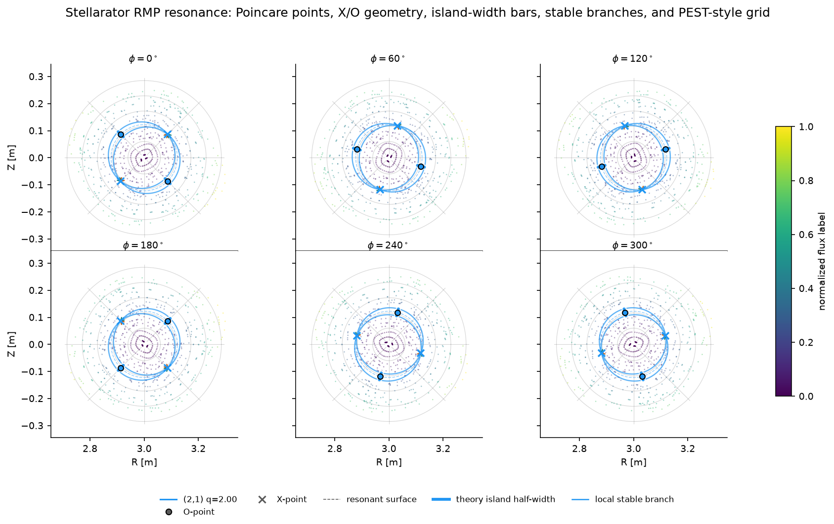
这个 notebook 是解析仿星器共振几何的主要公开工作流。它把两个原本分离的纯文本教程合并为一个可视化计算：

构建解析仿星器平衡并追踪 Poincaré 截面。
计算 RMP 的共振 Fourier 分量及其解析 X/O 不动点。
将原始截面点提升为几何对象：交点、不动点标记、共振面、O 点磁岛宽度条、局部稳定分支和坐标叠加层。
用 PEST 风格网格比较未扰动截面和受扰动截面。
汇总磁岛宽度、Chirikov 重叠和 \((m,n)\) 谱。
使用 pyna.plot 辅助函数生成现代化的多截面图。

这个 notebook 设计为在发布文档前于本地执行。GitHub Pages 会渲染保存的输出，而不是重新计算磁力线追踪。

[SETUP] 导入与发表图样式#

[1]:

import sys
import json
import pathlib
import numpy as np
import matplotlib
import matplotlib.pyplot as plt
from matplotlib.colors import Normalize

PROJECT_ROOT = None
for candidate in [pathlib.Path.cwd(), *pathlib.Path.cwd().parents]:
    if (candidate / 'pyna').is_dir() and (candidate / 'pyproject.toml').exists():
        PROJECT_ROOT = candidate
        break
if PROJECT_ROOT is not None and str(PROJECT_ROOT) not in sys.path:
    sys.path.insert(0, str(PROJECT_ROOT))

%matplotlib inline
from matplotlib_inline.backend_inline import set_matplotlib_formats
set_matplotlib_formats('png')

plt.rcParams.update({
    'font.family': 'DejaVu Sans',
    'font.size': 9,
    'axes.labelsize': 9,
    'axes.titlesize': 10,
    'figure.dpi': 150,
    'text.usetex': False,
    'axes.linewidth': 0.75,
    'axes.spines.top': False,
    'axes.spines.right': False,
    'figure.facecolor': 'white',
    'axes.facecolor': 'white',
})

from pyna.toroidal.equilibrium.stellarator import simple_stellarator
from pyna.toroidal.visual.RMP_spectrum import (
    find_resonant_components_analytic,
    radial_rmp_field_template,
    compose_magnetic_perturbations,
    circular_shell_divergence_diagnostic,
    fieldline_velocity_spectrum_on_circular_surface,
    rmp_nrmp_mode_rows,
    sample_stellarator_cylindrical_field,
    compare_cyna_fixed_points_for_component,
    deformed_circular_section_rz,
    deformed_surface_map_residual,
    project_fixed_points_to_deformed_surface,
    CoupledFixedPointSweep,
    plot_perturbation_order_summary,
    scan_nonresonant_residual_order,
    scan_coupled_fixed_point_sweep,
    scan_rmp_amplitude_order,
    scan_rmp_phase_order,
    scan_rmp_resolution_convergence,
    compute_mn_spectrum,
    plot_mn_heatmap,
    ISLAND_CMAPS,
)
from pyna.toroidal.perturbation_spectrum import (
    analyze_resonant_island_chains_multi_n,
    nardon_radial_perturbation,
    radial_perturbation_Fourier_spectrum,
)
from pyna.toroidal.visual.magnetic_spectrum import (
    PoincareRationalTrace,
    plot_radial_mode_heatmap,
    plot_rational_surface_map,
    plot_spectrum_bar3d,
    plot_spectrum_heatmap,
)
from pyna.topo.poincare import poincare_from_fieldlines, ToroidalSection
from pyna.plot import (
    draw_pest_grid,
    draw_poincare_points,
    draw_rmp_resonance_section,
    plot_rmp_resonance_sections,
)

print('Setup complete. numpy', np.__version__, '  matplotlib', matplotlib.__version__)

Setup complete. numpy 2.4.6   matplotlib 3.11.0

[EQ] 构建仿星器平衡#

我们使用一个解析的单螺旋度仿星器，参数为：

大半径 \(R_0 = 3.0\) m，小半径 \(r_0 = 0.3\) m，轴上磁场 \(B_0 = 2.5\) T
线性 \(q\) 剖面：\(q_0=1.5\)（磁轴）→ \(q_1=4.5\)（LCFS）
螺旋波纹：\((m_h, n_h) = (3,3)\)，\(\epsilon_h = 0.03\)

安全因子剖面 \(q(\psi) = q_0 + (q_1-q_0)\psi\) 覆盖区间 \([1.5, 4.5]\)，因此 \(q = 2/1, 3/1, 4/1\) 等共振位于等离子体内部。

[2]:

eq = simple_stellarator(
    R0=3.0, r0=0.3, B0=2.5,
    q0=1.5, q1=4.5,
    m_h=3, n_h=3, epsilon_h=0.03,
)
print(eq)
print(f'q range: [{eq.q0}, {eq.q1}]')
print(f'Resonant surface for (2,1): psi_res = {eq.resonant_psi(2,1)}')
print(f'Resonant surface for (4,2): psi_res = {eq.resonant_psi(4,2)}')
print(f'Resonant surface for (6,3): psi_res = {eq.resonant_psi(6,3)}')

# Convenience references
R0_eq = eq.R0
r0_eq = eq.r0

StellaratorSimple(R0=3.0 m, r0=0.3 m, B0=2.5 T, q=[1.5, 4.5], m_h=3, n_h=3, ε_h=0.03)
q range: [1.5, 4.5]
Resonant surface for (2,1): psi_res = [0.16666666666666666]
Resonant surface for (4,2): psi_res = [0.16666666666666666]
Resonant surface for (6,3): psi_res = [0.16666666666666666]

[RMP_NRMP_WORKFLOW] RMP/nRMP 分解#

通量面上的扰动模只有在与局部磁力线旋转变换比较之后才有明确意义。采用 Fourier 约定

\[F(\theta,\varphi)=\sum_{m,n} F_{mn}\exp[i(m\theta+n\varphi)],\]

局部失谐量为

\[\Delta_{mn}=m\iota+n, \qquad \iota=1/q.\]

部分	条件	几何效应	pyna 工作流
RMP	`abs(m*iota+n) <= tol`	产生磁岛链；X/O 点、O 点宽度条和分界线（separatrix）分支是一阶上有意义的对象	`find_resonant_components_analytic`, `compare_cyna_fixed_points_for_component`, `draw_rmp_resonance_section`
nRMP	对每个非共振模都有 `abs(m*iota+n) > tol`	所有非共振模相加后形成平滑的通量面形变和磁力线速度调制	`fieldline_velocity_spectrum_on_circular_surface`, `FieldlineVelocitySpectrum.nonresonant_response()`
混合谱	二者同时存在	共振岛几何叠加在总 nRMP 形变后的通量面上	`compose_magnetic_perturbations`, `nonresonant_response`, `rmp_nrmp_mode_rows` 用于诊断
验证	矢量场必须物理	非无散度模板可能产生伪拓扑	`radial_rmp_field_template`, `circular_shell_divergence_diagnostic`

关键差异在于：RMP 诊断聚焦共振模行，而 nRMP 响应是对所有非共振模行的完整求和：

\[\delta r(\theta,\varphi)=\sum_{m\iota+n\ne 0}\frac{F_{r,mn}}{i(m\iota+n)}\exp[i(m\theta+n\varphi)].\]

贡献表有助于排序和收敛检查，但模型本身是完整的非共振谱，而不是筛选出的最大分量。

[POINCARE_UNPERTURBED] \(\phi=0\) 处的未扰动 Poincaré 截面#

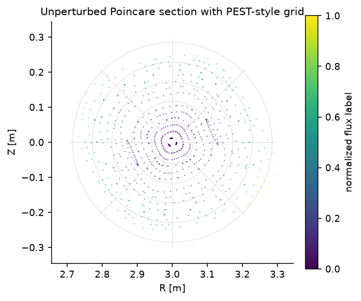
我们追踪未扰动平衡的磁力线，并记录它们在 \(\varphi=0\) 平面的穿越。结果是原始采样几何：有用，但还不是拓扑对象。后续单元会添加提升层，叠加共振面、X/O 标记、局部稳定分支和 PEST 风格坐标网格。

交点缓存到 pyna_output/poincare_unperturbed.json。

[3]:

CACHE_UNPERT = pathlib.Path('pyna_output/poincare_unperturbed.json')
CACHE_UNPERT.parent.mkdir(exist_ok=True)

if CACHE_UNPERT.exists():
    _d = json.loads(CACHE_UNPERT.read_text())
    R_cross_u = np.array(_d['R'])
    Z_cross_u = np.array(_d['Z'])
    print(f'Loaded from cache: {len(R_cross_u)} crossings')
else:
    n_fieldlines = 15
    n_turns = 50
    dt = 0.08
    t_max = n_turns * 2 * np.pi * eq.R0

    R_starts = np.linspace(eq.R0 + 0.04*eq.r0, eq.R0 + 0.92*eq.r0, n_fieldlines)
    start_pts = np.zeros((n_fieldlines, 3))
    start_pts[:, 0] = R_starts
    start_pts[:, 2] = 0.0

    sections_u = [ToroidalSection(phi0=0.0)]
    print(f'Tracing {n_fieldlines} field lines x {n_turns} turns (dt={dt}, t_max={t_max:.1f} m)...')

    pmap_u = poincare_from_fieldlines(
        eq.field_func,
        start_pts,
        sections_u,
        t_max=t_max,
        dt=dt,
    )
    arr_u = pmap_u.crossing_array(0)
    R_cross_u = arr_u[:, 0]
    Z_cross_u = arr_u[:, 1]
    print(f'Computed: {len(R_cross_u)} crossings. Caching...')
    CACHE_UNPERT.write_text(json.dumps({'R': R_cross_u.tolist(), 'Z': Z_cross_u.tolist()}))
    print('Cached.')

fig_u, ax_u = plt.subplots(figsize=(4.7, 4.3), constrained_layout=True)
draw_pest_grid(ax_u, eq, alpha=0.22)
psi_pts = np.clip(((R_cross_u - eq.R0)**2 + Z_cross_u**2) / eq.r0**2, 0, 1)
draw_poincare_points(
    ax_u,
    R_cross_u,
    Z_cross_u,
    values=psi_pts,
    cmap='viridis',
    point_size=1.8,
    alpha=0.50,
    rasterized=False,
)
sm_u = plt.cm.ScalarMappable(cmap='viridis', norm=Normalize(0, 1))
fig_u.colorbar(sm_u, ax=ax_u, label='normalized flux label', shrink=0.82)
lim = 1.15 * eq.r0
ax_u.set_xlim(eq.R0 - lim, eq.R0 + lim)
ax_u.set_ylim(-lim, lim)
ax_u.set_aspect('equal')
ax_u.set_xlabel('R [m]')
ax_u.set_ylabel('Z [m]')
ax_u.set_title('Unperturbed Poincare section with PEST-style grid')
plt.show()

Loaded from cache: 735 crossings

../../../../_images/notebooks_i18n_zh_tutorials_RMP_resonance_analysis_7_1.png

[RMP_FIELD] 定义并可视化 RMP 扰动场#

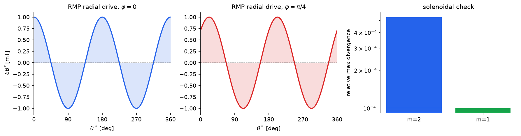
我们施加一个基模为 \((m,n)=(2,1)\)、幅度为 \(\delta B=1\) mT 的单模 RMP。面向用户的模板为

\[B_r = B_\mathrm{rmp}\cos(m\theta-n\varphi+\alpha),\]

但 radial_rmp_field_template 还会加入补偿性的极向/环向分量，使完整的柱坐标矢量场在局部圆壳度量下无散度。图中绘出的径向投影仍然是熟悉的共振驱动 \(\delta B^r\)。

同一个辅助函数支持重要的 m=1 分支；该情形需要环向分量，因为径向散度中包含与 \(\theta\) 无关的部分。

[4]:

base_m, base_n = 2, 1
B_rmp = 1e-3  # 1 mT

delta_B_RMP = radial_rmp_field_template(
    base_m,
    base_n,
    amplitude=B_rmp,
    phase=0.0,
    axis_R=eq.R0,
)

psi_res_21 = eq.resonant_psi(2, 1)[0]
r_res_21 = np.sqrt(psi_res_21) * eq.r0
print(f'q=2/1 resonant surface: psi={psi_res_21:.3f}, r={r_res_21*100:.1f} cm')
print(f'delta_B/B0 = {B_rmp/eq.B0*100:.3f}%')

r_check = np.linspace(0.08, 0.28, 7)
div_m2 = circular_shell_divergence_diagnostic(
    delta_B_RMP,
    axis_R=eq.R0,
    r_values=r_check,
    n_theta=192,
    n_phi=192,
)
delta_B_m1_demo = radial_rmp_field_template(
    1,
    1,
    amplitude=B_rmp,
    phase=0.35,
    axis_R=eq.R0,
)
div_m1 = circular_shell_divergence_diagnostic(
    delta_B_m1_demo,
    axis_R=eq.R0,
    r_values=r_check,
    n_theta=192,
    n_phi=192,
)

print('Divergence diagnostics for the full vector perturbation:')
print('{:<8} {:>12} {:>12} {:>12}'.format('mode', 'max |div|', 'rms |div|', 'rel max'))
for label, diag in [('m=2', div_m2), ('m=1', div_m1)]:
    print(f'{label:<8} {diag.max_abs:12.3e} {diag.rms:12.3e} {diag.relative_max:12.3e}')

theta_arr = np.linspace(0, 2*np.pi, 240)
R_res = eq.R0 + r_res_21 * np.cos(theta_arr)
Z_res = r_res_21 * np.sin(theta_arr)

fig_rmp, axes_rmp = plt.subplots(1, 3, figsize=(11.8, 3.0), constrained_layout=True)
for ax, phi_val, phi_label, color in [
    (axes_rmp[0], 0.0, r'$\varphi=0$', '#2563eb'),
    (axes_rmp[1], np.pi/4, r'$\varphi=\pi/4$', '#dc2626'),
]:
    BR, BZ, _ = delta_B_RMP(R_res, Z_res, phi_val)
    dBpsi = BR*np.cos(theta_arr) + BZ*np.sin(theta_arr)
    ax.plot(np.degrees(theta_arr), dBpsi * 1e3, color=color, linewidth=1.8)
    ax.fill_between(np.degrees(theta_arr), 0, dBpsi * 1e3, color=color, alpha=0.16, linewidth=0)
    ax.axhline(0, color='0.25', lw=0.7, linestyle='--')
    ax.set_xlabel(r'$\theta^*$ [deg]')
    ax.set_title(f'RMP radial drive, {phi_label}')
    ax.set_xlim(0, 360)
    ax.set_xticks([0, 90, 180, 270, 360])
axes_rmp[0].set_ylabel(r'$\delta B^r$ [mT]')

axes_rmp[2].bar(['m=2', 'm=1'], [div_m2.relative_max, div_m1.relative_max], color=['#2563eb', '#16a34a'])
axes_rmp[2].set_yscale('log')
axes_rmp[2].set_ylabel('relative max divergence')
axes_rmp[2].set_title('solenoidal check')
axes_rmp[2].grid(True, axis='y', alpha=0.25)
plt.show()
print('Divergence-free RMP field defined and visualised.')

q=2/1 resonant surface: psi=0.167, r=12.2 cm
delta_B/B0 = 0.040%
Divergence diagnostics for the full vector perturbation:
mode        max |div|    rms |div|      rel max
m=2         6.642e-06    3.148e-06    5.300e-04
m=1         1.804e-06    7.949e-07    9.946e-05

../../../../_images/notebooks_i18n_zh_tutorials_RMP_resonance_analysis_9_1.png

Divergence-free RMP field defined and visualised.

[M1_RMP] m=1 相位控制小案例#

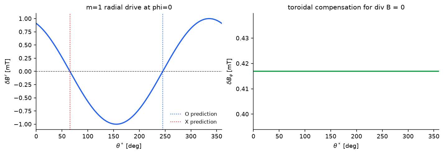
m=1 扰动足够常见，不应被当作边缘情形处理。这里同一个无散模板在简单的 q=1 平衡中驱动 (1,1) 共振。我们在一次短计算中验证三件事：场在数值上无散，提取出的 b_{1,-1} 相位跟随模板相位，并且预测的 O/X 点落在径向驱动的零交叉上。

[5]:

eq_m1 = simple_stellarator(
    R0=eq.R0,
    r0=eq.r0,
    B0=eq.B0,
    q0=0.75,
    q1=1.25,
    m_h=eq.m_h,
    n_h=eq.n_h,
    epsilon_h=0.0,
)
m1_phase = 0.43
delta_B_m1 = radial_rmp_field_template(
    1,
    1,
    amplitude=B_rmp,
    phase=m1_phase,
    axis_R=eq_m1.R0,
)
psi_res_m1 = eq_m1.resonant_psi(1, 1)[0]
r_res_m1 = np.sqrt(psi_res_m1) * eq_m1.r0
m1_diag = circular_shell_divergence_diagnostic(
    delta_B_m1,
    axis_R=eq_m1.R0,
    r_values=np.linspace(0.08, 0.28, 7),
    n_theta=192,
    n_phi=192,
)
component_m1 = find_resonant_components_analytic(
    eq_m1,
    delta_B_m1,
    base_m=1,
    base_n=1,
    max_harmonic=1,
    n_theta=128,
    n_phi=64,
    min_amplitude=1e-16,
)[0]

print(f'm=1 resonant surface: psi={psi_res_m1:.3f}, r={r_res_m1*100:.1f} cm')
print(f'arg b_(1,-1) = {np.angle(component_m1.b_mn):.6f} rad, template phase = {m1_phase:.6f} rad')
print(f'|b_(1,-1)| = {abs(component_m1.b_mn):.3e} T, expected about B_rmp/2 = {0.5*B_rmp:.3e} T')
print(f'm=1 divergence relative max = {m1_diag.relative_max:.3e}')
print(f'O-point theta = {np.degrees(component_m1.opoint_theta):.2f} deg')
print(f'X-point theta = {np.degrees(component_m1.xpoint_theta):.2f} deg')

theta_m1 = np.linspace(0, 2*np.pi, 361)
R_m1 = eq_m1.R0 + r_res_m1*np.cos(theta_m1)
Z_m1 = r_res_m1*np.sin(theta_m1)
BR_m1, BZ_m1, Bphi_m1 = delta_B_m1(R_m1, Z_m1, 0.0)
dBr_m1 = BR_m1*np.cos(theta_m1) + BZ_m1*np.sin(theta_m1)

fig_m1, (ax_m1, ax_m1b) = plt.subplots(1, 2, figsize=(9.4, 3.2), constrained_layout=True)
ax_m1.plot(np.degrees(theta_m1), dBr_m1*1e3, color='#2563eb', lw=1.8)
ax_m1.axhline(0, color='0.25', lw=0.7, ls='--')
ax_m1.axvline(np.degrees(component_m1.opoint_theta), color='#2563eb', lw=1.1, ls=':', label='O prediction')
ax_m1.axvline(np.degrees(component_m1.xpoint_theta), color='#dc2626', lw=1.1, ls=':', label='X prediction')
ax_m1.set_xlim(0, 360)
ax_m1.set_xlabel(r'$\theta^*$ [deg]')
ax_m1.set_ylabel(r'$\delta B^r$ [mT]')
ax_m1.set_title('m=1 radial drive at phi=0')
ax_m1.legend(frameon=False, fontsize=8)

ax_m1b.plot(np.degrees(theta_m1), Bphi_m1*1e3, color='#16a34a', lw=1.8)
ax_m1b.set_xlim(0, 360)
ax_m1b.set_xlabel(r'$\theta^*$ [deg]')
ax_m1b.set_ylabel(r'$\delta B_\varphi$ [mT]')
ax_m1b.set_title('toroidal compensation for div B = 0')
plt.show()

  k=1: (1,1) ψ_res=0.500 q_res=1.000 |b_mn|=5.000e-04 phase_arg=24.6° w_ψ=0.1265 (2.68 cm) θ_O=245.4° θ_X=65.4°
m=1 resonant surface: psi=0.500, r=21.2 cm
arg b_(1,-1) = 0.430000 rad, template phase = 0.430000 rad
|b_(1,-1)| = 5.000e-04 T, expected about B_rmp/2 = 5.000e-04 T
m=1 divergence relative max = 9.946e-05
O-point theta = 245.36 deg
X-point theta = 65.36 deg

../../../../_images/notebooks_i18n_zh_tutorials_RMP_resonance_analysis_11_1.png

[RESONANT_COMPONENTS] 寻找共振 Fourier 分量#

我们在每个共振通量面上用二维 FFT 分解 RMP 场，并提取共振 \((m_k, n_k) = k\times(2,1)\) 谐波的幅度。磁岛半宽由 Rutherford 公式给出：

\[w_\psi = 4\sqrt{\frac{|b_{mn}|}{m|\partial q/\partial\psi|}}\]

结果缓存到 pyna_output/rmp_components.json。

[6]:

CACHE_COMP = pathlib.Path('pyna_output/rmp_components.json')
CACHE_COMP.parent.mkdir(exist_ok=True)

print('Computing resonant components (n_theta=32, n_phi=16)...')
components = find_resonant_components_analytic(
    eq, delta_B_RMP, base_m=base_m, base_n=base_n,
    max_harmonic=3, n_theta=32, n_phi=16,
)
print(f'Found {len(components)} resonant components.')

# Cache as JSON
_comp_data = [{
    'm': c.m, 'n': c.n, 'harmonic_order': c.harmonic_order,
    'b_mn_real': float(c.b_mn.real), 'b_mn_imag': float(c.b_mn.imag),
    'psi_res': float(c.psi_res), 'q_res': float(c.q_res),
    'half_width_psi': float(c.half_width_psi),
    'half_width_r': float(c.half_width_r),
    'opoint_theta': float(c.opoint_theta),
    'xpoint_theta': float(c.xpoint_theta),
    'q_prime_sign': int(c.q_prime_sign),
} for c in components]
CACHE_COMP.write_text(json.dumps(_comp_data, indent=2))
print('Cached to', CACHE_COMP)

# Print table
print()
print(f'{"k":>3}  {"(m,n)":>8}  {"psi_res":>8}  {"q_res":>6}  {"b_mn|":>10}  {"w_psi":>8}  {"w_r (cm)":>10}  {"theta_O":>8}  {"theta_X":>8}')
print('-'*80)
for c in components:
    print(f'{c.harmonic_order:>3}  ({c.m},{c.n}){"":>4}  {c.psi_res:>8.4f}  {c.q_res:>6.3f}  {abs(c.b_mn):>10.3e}  {c.half_width_psi:>8.4f}  {c.half_width_r*100:>10.2f}  {np.degrees(c.opoint_theta):>8.1f}  {np.degrees(c.xpoint_theta):>8.1f}')

Computing resonant components (n_theta=32, n_phi=16)...
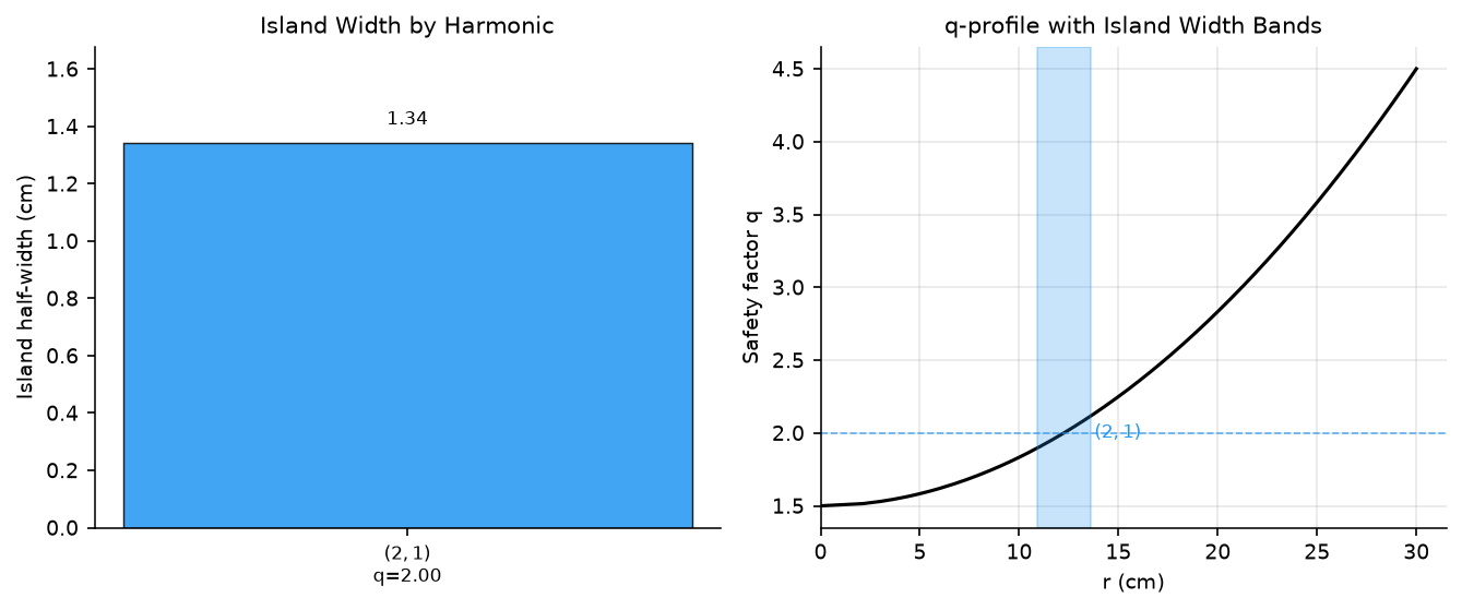
  k=1: (2,1) ψ_res=0.167 q_res=2.000 |b_mn|=5.000e-04 phase_arg=-0.0° w_ψ=0.0365 (1.34 cm) θ_O=135.0° θ_X=45.0°
  k=2: (4,2) — |b_mn|=4.57e-21 below threshold
  k=3: (6,3) — |b_mn|=1.98e-20 below threshold
Found 1 resonant components.
Cached to pyna_output/rmp_components.json

  k     (m,n)   psi_res   q_res       b_mn|     w_psi    w_r (cm)   theta_O   theta_X
--------------------------------------------------------------------------------
  1  (2,1)        0.1667   2.000   5.000e-04    0.0365        1.34     135.0      45.0

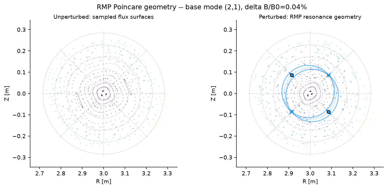
[POINCARE_PERTURBED] 几何提升：交点 -> X/O 点 -> 流形#

受扰动追踪给出采样的 Poincaré 点。解析 RMP 谱给出不动点和磁岛宽度预测。pyna.plot.draw_rmp_resonance_section 将它们合并成一个截面几何：

按通量标签着色的 Poincaré 点；
PEST 风格的 \((S,\theta^*)\) 网格线；
每个谐波的共振面；
由解析不动点公式给出的 O 点和 X 点；
由共振 Fourier 幅度决定长度的 O 点径向条；
从 X 点产生的局部稳定分界线（separatrix）分支。

这与通用几何工作流使用的是同一个提升思想：在显式模型或诊断证明提升合理之前，原始样本与持久几何对象及叠加层保持区分。

[7]:

# Perturbed field_func
# --------------------
def field_func_perturbed(rzphi_1d):
    """Unit-tangent dRZphi/ds for the field-line ODE with RMP added."""
    rzphi_1d = np.asarray(rzphi_1d, dtype=float)
    R, Z, phi = rzphi_1d[0], rzphi_1d[1], rzphi_1d[2]
    theta = np.arctan2(Z, R - R0_eq)
    psi = eq.psi_ax(R, Z)
    q = float(eq.q_of_psi(psi))
    r_minor = np.sqrt((R - R0_eq)**2 + Z**2)
    B_phi = eq.B0 * eq.R0 / R
    B_pol = B_phi * r_minor / (R * max(abs(q), 1e-3))
    if r_minor > 1e-10:
        BR0 = -B_pol * np.sin(theta)
        BZ0 =  B_pol * np.cos(theta)
    else:
        BR0 = BZ0 = 0.0
    delta_BR_eq = eq.epsilon_h * eq.B0 * psi * np.cos(eq.m_h * theta - eq.n_h * phi)
    db = delta_B_RMP(R, Z, phi)
    BR_tot = BR0 + delta_BR_eq + db[0]
    BZ_tot = BZ0 + db[1]
    B_phi_tot = B_phi + db[2]
    B_mag = np.sqrt(BR_tot**2 + BZ_tot**2 + B_phi_tot**2) + 1e-30
    return np.array([BR_tot/B_mag, BZ_tot/B_mag, B_phi_tot/(R*B_mag)])

CACHE_PERT = pathlib.Path('pyna_output/poincare_perturbed_divfree.json')
CACHE_PERT.parent.mkdir(exist_ok=True)

phi_sections_deg = [0, 60, 120, 180, 240, 300]
phi_sections = np.array(phi_sections_deg) * np.pi / 180.0

if CACHE_PERT.exists():
    _d = json.loads(CACHE_PERT.read_text())
    all_sections_data = _d['sections']
    print(f'Loaded perturbed Poincare from cache ({len(all_sections_data)} sections).')
else:
    sections_p = [ToroidalSection(phi0=ph) for ph in phi_sections]
    n_fieldlines, n_turns, dt = 15, 50, 0.08
    t_max = n_turns * 2 * np.pi * eq.R0
    start_pts = np.zeros((n_fieldlines, 3))
    start_pts[:, 0] = np.linspace(eq.R0 + 0.04*eq.r0, eq.R0 + 0.92*eq.r0, n_fieldlines)

    print(f'Tracing {n_fieldlines} field lines x {n_turns} turns (t_max={t_max:.1f} m)...')
    pmap_p = poincare_from_fieldlines(field_func_perturbed, start_pts, sections_p, t_max=t_max, dt=dt)
    all_sections_data = []
    for i_sec, phi_deg in enumerate(phi_sections_deg):
        arr = pmap_p.crossing_array(i_sec)
        print(f'  phi={phi_deg} deg: {len(arr)} crossings')
        all_sections_data.append({'R': arr[:, 0].tolist() if len(arr) else [], 'Z': arr[:, 1].tolist() if len(arr) else []})
    CACHE_PERT.write_text(json.dumps({'phi_sections_deg': phi_sections_deg, 'sections': all_sections_data}))
    print('Computed and cached.')

R_cross_p0 = np.array(all_sections_data[0]['R'])
Z_cross_p0 = np.array(all_sections_data[0]['Z'])
print(f'phi=0 section: {len(R_cross_p0)} crossings')

fig2, (axL, axR) = plt.subplots(1, 2, figsize=(9.4, 4.2), constrained_layout=True)

# The low-level plot layers are independently selectable by name.
draw_rmp_resonance_section(
    axL,
    R_cross_u,
    Z_cross_u,
    eq=eq,
    components=[],
    phi=0.0,
    title='Unperturbed: sampled flux surfaces',
    overlays=('pest_grid', 'poincare'),
    point_size=1.8,
    point_alpha=0.46,
)
draw_rmp_resonance_section(
    axR,
    R_cross_p0,
    Z_cross_p0,
    eq=eq,
    components=components,
    phi=0.0,
    colors=ISLAND_CMAPS,
    title='Perturbed: RMP resonance geometry',
    overlays=('pest_grid', 'poincare', 'resonant_surfaces', 'stable_branches', 'island_width_bars', 'xo'),
    point_size=1.8,
    point_alpha=0.46,
)

fig2.suptitle(
    f'RMP Poincare geometry -- base mode ({base_m},{base_n}), '
    f'delta B/B0={B_rmp/eq.B0*100:.2f}%',
    fontsize=11,
)
plt.show()

Loaded perturbed Poincare from cache (6 sections).
phi=0 section: 735 crossings

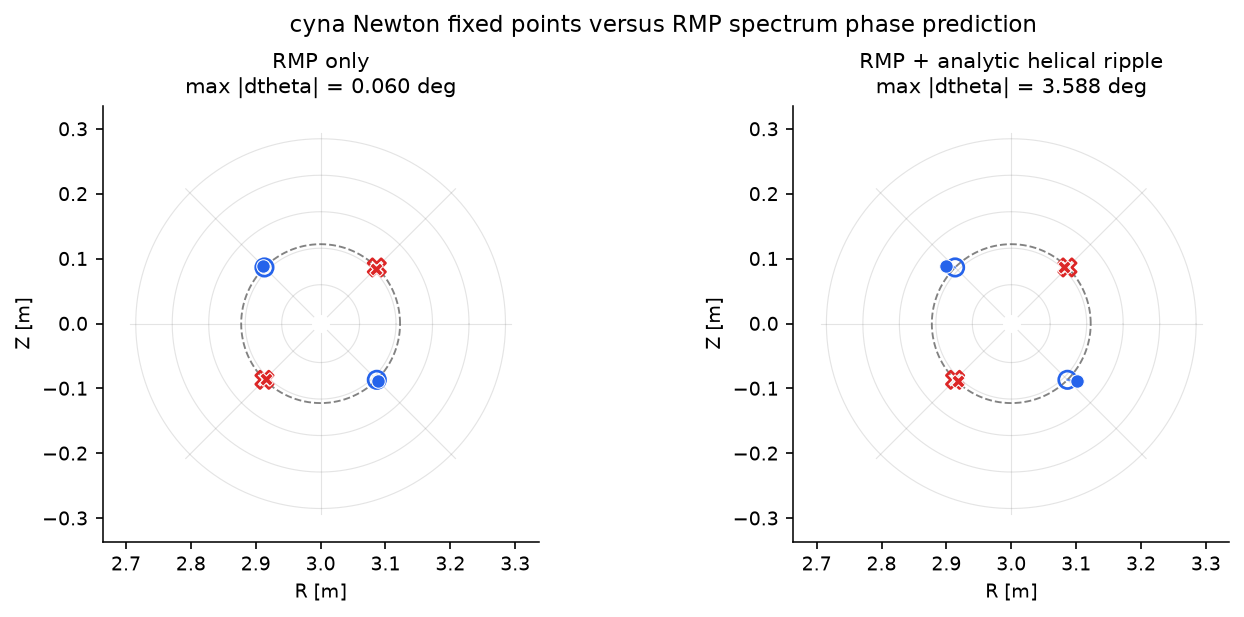
../../../../_images/notebooks_i18n_zh_tutorials_RMP_resonance_analysis_15_1.png

[CYNA_FIXED_POINTS] Newton 不动点与 RMP 谱相位对比#

RMP 谱预测一阶 O/X 点相位。这里我们使用加速的 cyna Newton 映射，将这些种子细化为真正的周期轨道不动点，然后测量相位误差。仅含 RMP 的情形是代码健全性检查；加入解析螺旋波纹后，则展示一阶谱有意忽略的有限幅度/模型位移。

[8]:

# Build a physical cylindrical field for cyna and compare Newton fixed points.
def row_newton_theta_deg(row, eq_case):
    axis_R, axis_Z = eq_case.magnetic_axis
    theta = np.arctan2(row.newton_Z - axis_Z, row.newton_R - axis_R) % (2*np.pi)
    return float(np.degrees(theta))


cyna_rows_by_case = {}
cyna_eq_by_case = {}
if components:
    eq_rmp_only = simple_stellarator(
        R0=eq.R0, r0=eq.r0, B0=eq.B0,
        q0=eq.q0, q1=eq.q1,
        m_h=eq.m_h, n_h=eq.n_h, epsilon_h=0.0,
    )
    try:
        for case_label, eq_case in [
            ('RMP only', eq_rmp_only),
            ('RMP + analytic helical ripple', eq),
        ]:
            print(f'Building cyna field: {case_label}')
            field_case = sample_stellarator_cylindrical_field(
                eq_case,
                delta_B_RMP,
                nR=128,
                nPhi=128,
                label=f'analytic_rmp_for_cyna_{case_label.replace(" ", "_").lower()}',
            )
            rows = compare_cyna_fixed_points_for_component(
                field_case,
                components[0],
                eq_case,
                DPhi=0.015,
                max_iter=80,
                tol=1e-11,
                n_threads=4,
            )
            cyna_rows_by_case[case_label] = rows
            cyna_eq_by_case[case_label] = eq_case
    except ImportError as exc:
        print('cyna fixed-point comparison skipped:', exc)

if cyna_rows_by_case:
    print()
    header = '{:<30} {:>4} {:>6} {:>9} {:>9} {:>10} {:>11} {:>11} {:>11}'.format(
        'case', 'kind', 'branch', 'theta*', 'theta_N', 'dtheta', 'm*dtheta', 'dr [cm]', 'residual'
    )
    print(header)
    print('-' * len(header))
    for case_label, rows in cyna_rows_by_case.items():
        eq_case = cyna_eq_by_case[case_label]
        for row in rows:
            theta_n = row_newton_theta_deg(row, eq_case)
            print('{:<30} {:>4} {:>6d} {:>9.3f} {:>9.3f} {:>10.4f} {:>11.4f} {:>11.4f} {:>11.1e}'.format(
                case_label,
                row.predicted_kind + '/' + (row.newton_kind or '?'),
                row.branch,
                row.predicted_theta_deg,
                theta_n,
                row.theta_error_deg,
                row.helical_phase_error_deg,
                row.radial_error_cm,
                row.residual,
            ))
        max_dtheta = max(abs(row.theta_error_deg) for row in rows)
        max_helical = max(abs(row.helical_phase_error_deg) for row in rows)
        print(f'  -> {case_label}: max |dtheta|={max_dtheta:.4f} deg, max |m*dtheta|={max_helical:.4f} deg')

if cyna_rows_by_case:
    fig_cmp, axes_cmp = plt.subplots(1, len(cyna_rows_by_case), figsize=(9.2, 4.0), constrained_layout=True)
    axes_cmp = np.atleast_1d(axes_cmp)
    for ax, (case_label, rows) in zip(axes_cmp, cyna_rows_by_case.items()):
        eq_case = cyna_eq_by_case[case_label]
        draw_pest_grid(ax, eq_case, alpha=0.18)
        r_res = np.sqrt(components[0].psi_res) * eq_case.r0
        theta_ring = np.linspace(0, 2*np.pi, 361)
        ax.plot(eq_case.R0 + r_res*np.cos(theta_ring), r_res*np.sin(theta_ring),
                color='0.25', lw=0.9, ls='--', alpha=0.65)
        for row in rows:
            color = '#2563eb' if row.predicted_kind == 'O' else '#dc2626'
            marker = 'o' if row.predicted_kind == 'O' else 'X'
            ax.plot([row.predicted_R, row.newton_R], [row.predicted_Z, row.newton_Z],
                    color=color, lw=1.0, alpha=0.65)
            ax.scatter(row.predicted_R, row.predicted_Z, marker=marker, s=70,
                       facecolors='none', edgecolors=color, linewidths=1.3, zorder=5)
            ax.scatter(row.newton_R, row.newton_Z, marker=marker, s=42,
                       color=color, edgecolors='white', linewidths=0.5, zorder=6)
        lim = 1.12 * eq_case.r0
        ax.set_xlim(eq_case.R0 - lim, eq_case.R0 + lim)
        ax.set_ylim(-lim, lim)
        ax.set_aspect('equal')
        ax.set_xlabel('R [m]')
        ax.set_ylabel('Z [m]')
        max_dtheta = max(abs(row.theta_error_deg) for row in rows)
        ax.set_title(f'{case_label}\nmax |dtheta| = {max_dtheta:.3f} deg')
    fig_cmp.suptitle('cyna Newton fixed points versus RMP spectrum phase prediction', fontsize=11)
    plt.show()

Building cyna field: RMP only
Building cyna field: RMP + analytic helical ripple

case                           kind branch    theta*   theta_N     dtheta    m*dtheta     dr [cm]    residual
-------------------------------------------------------------------------------------------------------------
RMP only                        O/O      0   315.000   314.940    -0.0602     -0.1203      0.2298     1.4e-14
RMP only                        O/O      1   135.000   135.059     0.0588      0.1176      0.2303     9.2e-15
RMP only                        X/X      0    45.000    44.940    -0.0600     -0.1200     -0.2520     4.7e-14
RMP only                        X/X      1   225.000   225.059     0.0588      0.1176     -0.2515     1.7e-14
  -> RMP only: max |dtheta|=0.0602 deg, max |m*dtheta|=0.1203 deg
RMP + analytic helical ripple   O/O      0   315.000   318.588     3.5877      7.1754      1.2050     5.0e-12
RMP + analytic helical ripple   O/O      1   135.000   138.420     3.4195      6.8391      1.1869     2.2e-15
RMP + analytic helical ripple   X/X      0    45.000    47.043     2.0428      4.0857     -0.2143     2.7e-12
RMP + analytic helical ripple   X/X      1   225.000   226.940     1.9400      3.8801     -0.2445     2.3e-12
  -> RMP + analytic helical ripple: max |dtheta|=3.5877 deg, max |m*dtheta|=7.1754 deg

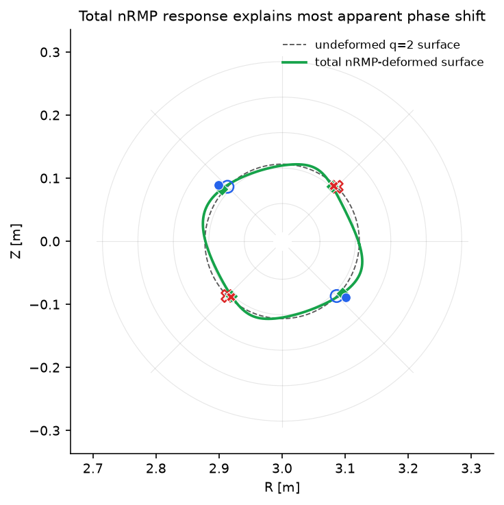
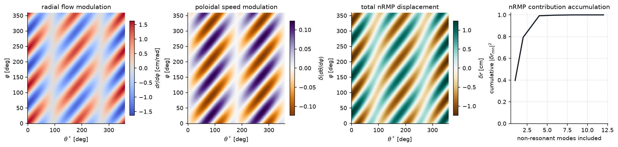
../../../../_images/notebooks_i18n_zh_tutorials_RMP_resonance_analysis_17_1.png

[NONRESONANT_DEFORMATION] 作为通量面形变的非共振波纹#

这个解析平衡中的螺旋波纹不是产生 (m,n)=(2,1) 磁岛的共振 RMP 分量。它仍然会改变附近通量面的几何。如果把 Newton 不动点与未形变的圆形通量面比较，这种平滑位移会表现为人为的相位误差。

这里我们采样螺旋波纹对磁力线 ODE 的贡献，

\[\frac{dr}{d\phi}=F_r(\theta,\phi), \qquad \frac{d\theta}{d\phi}=\iota+F_\theta(\theta,\phi),\]

对 F_r 和 F_theta 做 Fourier 变换，并为每个非共振系数求解非共振同调方程。响应对象同时保留总形变和贡献排序；排序是诊断信息，而下文使用的形变是完整求和后的 nRMP 响应。

[9]:

def helical_ripple_delta_B(eq_case):
    """Return the analytic helical-ripple contribution used by simple_stellarator."""
    def delta_B_helical(R, Z, phi):
        R_arr = np.asarray(R, dtype=float)
        Z_arr = np.asarray(Z, dtype=float)
        phi_arr = np.asarray(phi, dtype=float)
        theta = np.arctan2(Z_arr, R_arr - eq_case.R0)
        psi = eq_case.psi_ax(R_arr, Z_arr)
        dBR = eq_case.epsilon_h * eq_case.B0 * psi * np.cos(eq_case.m_h * theta - eq_case.n_h * phi_arr)
        return np.array([
            dBR,
            np.zeros_like(dBR, dtype=float),
            np.zeros_like(dBR, dtype=float),
        ])
    return delta_B_helical


def helical_velocity_response(eq_case, psi_res, n_theta=256, n_phi=256, include_shear=False):
    velocity = fieldline_velocity_spectrum_on_circular_surface(
        eq_case,
        helical_ripple_delta_B(eq_case),
        psi_res,
        n_theta=n_theta,
        n_phi=n_phi,
        m_max=8,
        n_max=8,
        min_amplitude=1e-12,
    )
    return velocity.nonresonant_response(include_shear=include_shear)


def helical_velocity_deformation(eq_case, psi_res, n_theta=256, n_phi=256, include_shear=False):
    response = helical_velocity_response(
        eq_case,
        psi_res,
        n_theta=n_theta,
        n_phi=n_phi,
        include_shear=include_shear,
    )
    return response.deformation, response.velocity.r_minor, response.velocity


case_label = 'RMP + analytic helical ripple'
if components and case_label in cyna_rows_by_case:
    rows = cyna_rows_by_case[case_label]
    eq_case = cyna_eq_by_case[case_label]
    response_helical = helical_velocity_response(eq_case, components[0].psi_res)
    deformation = response_helical.deformation
    velocity_helical = response_helical.velocity
    r_res = velocity_helical.r_minor
    projected_rows = project_fixed_points_to_deformed_surface(
        rows,
        eq_case,
        deformation,
        r_minor=r_res,
        theta_window=0.35,
    )

    print(
        'nRMP total response uses '
        f'{response_helical.n_nonresonant_modes} non-resonant modes '
        f'and excludes {response_helical.n_resonant_modes} resonant modes.'
    )
    print('Largest nRMP response contributors; these rank the sum but do not replace it:')
    print('{:>8} {:>12} {:>14} {:>14}'.format('(m,n)', 'detuning', '|delta_r_mn| cm', 'cum frac'))
    for contrib in response_helical.contribution_rows(top=6):
        print('({:>2d},{:>2d}) {:>12.3e} {:>14.4f} {:>14.3f}'.format(
            contrib.m,
            contrib.n,
            contrib.detuning,
            100.0 * contrib.radial_response_weight,
            contrib.cumulative_fraction,
        ))
    print()

    raw_max = max(abs(row.theta_error_deg) for row in rows)
    corrected_max = max(abs(row.theta_error_deg) for row in projected_rows)
    nearest_max = max(row.distance_cm for row in projected_rows)
    print(f'Raw circular-surface max |dtheta|:       {raw_max:.4f} deg')
    print(f'Deformed-surface-coordinate max |dtheta|: {corrected_max:.4f} deg')
    print(f'Max Newton-to-deformed-section distance:  {nearest_max:.3f} cm')
    print()
    header = '{:<4} {:>6} {:>12} {:>16} {:>13}'.format(
        'kind', 'branch', 'raw dtheta', 'deformed dtheta', 'distance [cm]'
    )
    print(header)
    print('-' * len(header))
    for row, proj in zip(rows, projected_rows):
        print('{:<4} {:>6d} {:>12.4f} {:>16.4f} {:>13.3f}'.format(
            row.predicted_kind,
            row.branch,
            row.theta_error_deg,
            proj.theta_error_deg,
            proj.distance_cm,
        ))

    theta_line = np.linspace(0.0, 2*np.pi, 721)
    R_circ = eq_case.R0 + r_res*np.cos(theta_line)
    Z_circ = r_res*np.sin(theta_line)
    R_def, Z_def = deformed_circular_section_rz(eq_case, r_res, deformation, theta_line)

    fig_def, ax_def = plt.subplots(figsize=(5.2, 4.8), constrained_layout=True)
    draw_pest_grid(ax_def, eq_case, alpha=0.16)
    ax_def.plot(R_circ, Z_circ, color='0.35', lw=0.9, ls='--', label='undeformed q=2 surface')
    ax_def.plot(R_def, Z_def, color='#16a34a', lw=1.8, label='total nRMP-deformed surface')

    for row, proj in zip(rows, projected_rows):
        color = '#2563eb' if row.predicted_kind == 'O' else '#dc2626'
        marker = 'o' if row.predicted_kind == 'O' else 'X'
        ax_def.plot([row.predicted_R, row.newton_R], [row.predicted_Z, row.newton_Z],
                    color=color, lw=0.8, alpha=0.35)
        ax_def.plot([proj.closest_R, row.newton_R], [proj.closest_Z, row.newton_Z],
                    color=color, lw=1.1, ls=':', alpha=0.9)
        ax_def.scatter(row.predicted_R, row.predicted_Z, marker=marker, s=72,
                       facecolors='none', edgecolors=color, linewidths=1.2, zorder=5)
        ax_def.scatter(proj.closest_R, proj.closest_Z, marker='D', s=42,
                       color='#16a34a', edgecolors='white', linewidths=0.45, zorder=6)
        ax_def.scatter(row.newton_R, row.newton_Z, marker=marker, s=44,
                       color=color, edgecolors='white', linewidths=0.5, zorder=7)

    lim = 1.12 * eq_case.r0
    ax_def.set_xlim(eq_case.R0 - lim, eq_case.R0 + lim)
    ax_def.set_ylim(-lim, lim)
    ax_def.set_aspect('equal')
    ax_def.set_xlabel('R [m]')
    ax_def.set_ylabel('Z [m]')
    ax_def.set_title('Total nRMP response explains most apparent phase shift')
    ax_def.legend(frameon=False, loc='upper right', fontsize=8)
    plt.show()

    TT_h, PP_h, dr_h, dtheta_h = response_helical.real_fields()
    counts_h, cumulative_h = response_helical.cumulative_contribution()
    theta_deg_h = np.degrees(velocity_helical.theta)
    phi_deg_h = np.degrees(velocity_helical.phi)
    fig_flow, axes_flow = plt.subplots(1, 4, figsize=(13.8, 3.2), constrained_layout=True)
    panels = [
        (velocity_helical.radial_velocity * 100.0, r'$dr/d\varphi$ [cm/rad]', 'radial flow modulation', 'coolwarm'),
        (velocity_helical.poloidal_velocity, r'$\delta(d\theta/d\varphi)$', 'poloidal speed modulation', 'PuOr'),
        (dr_h * 100.0, r'$\delta r$ [cm]', 'total nRMP displacement', 'BrBG'),
    ]
    for ax, (data, cbar_label, title, cmap) in zip(axes_flow[:3], panels):
        vmax = np.nanmax(np.abs(data))
        im = ax.pcolormesh(
            theta_deg_h,
            phi_deg_h,
            data,
            shading='auto',
            cmap=cmap,
            vmin=-vmax,
            vmax=vmax,
        )
        ax.set_xlabel(r'$\theta^*$ [deg]')
        ax.set_ylabel(r'$\varphi$ [deg]')
        ax.set_title(title)
        fig_flow.colorbar(im, ax=ax, label=cbar_label, shrink=0.85)
    axes_flow[3].plot(counts_h, cumulative_h, color='#111827', lw=1.8)
    axes_flow[3].set_ylim(0, 1.02)
    axes_flow[3].set_xlabel('non-resonant modes included')
    axes_flow[3].set_ylabel(r'cumulative $|\delta r_{mn}|^2$')
    axes_flow[3].set_title('nRMP contribution accumulation')
    axes_flow[3].grid(True, alpha=0.25)
    plt.show()
else:
    print('Non-resonant deformation check skipped because cyna rows are unavailable.')

nRMP total response uses 12 non-resonant modes and excludes 2 resonant modes.
Largest nRMP response contributors; these rank the sum but do not replace it:
   (m,n)     detuning |delta_r_mn| cm       cum frac
(-4, 3)    1.000e+00         0.3755          0.397
( 4,-3)   -1.000e+00         0.3755          0.794
(-2, 3)    2.000e+00         0.1877          0.893
( 2,-3)   -2.000e+00         0.1877          0.992
(-5, 3)    5.000e-01         0.0306          0.995
( 5,-3)   -5.000e-01         0.0306          0.997

Raw circular-surface max |dtheta|:       3.5877 deg
Deformed-surface-coordinate max |dtheta|: 1.4748 deg
Max Newton-to-deformed-section distance:  0.822 cm

kind branch   raw dtheta  deformed dtheta distance [cm]
-------------------------------------------------------
O         0       3.5877           0.6159         0.822
O         1       3.4195           0.7933         0.783
X         0       2.0428          -1.4748         0.250
X         1       1.9400          -1.1567         0.196

../../../../_images/notebooks_i18n_zh_tutorials_RMP_resonance_analysis_19_1.png

../../../../_images/notebooks_i18n_zh_tutorials_RMP_resonance_analysis_19_2.png

[MIXED_SPECTRUM] 单个通量面上的混合 RMP/nRMP 工作流#

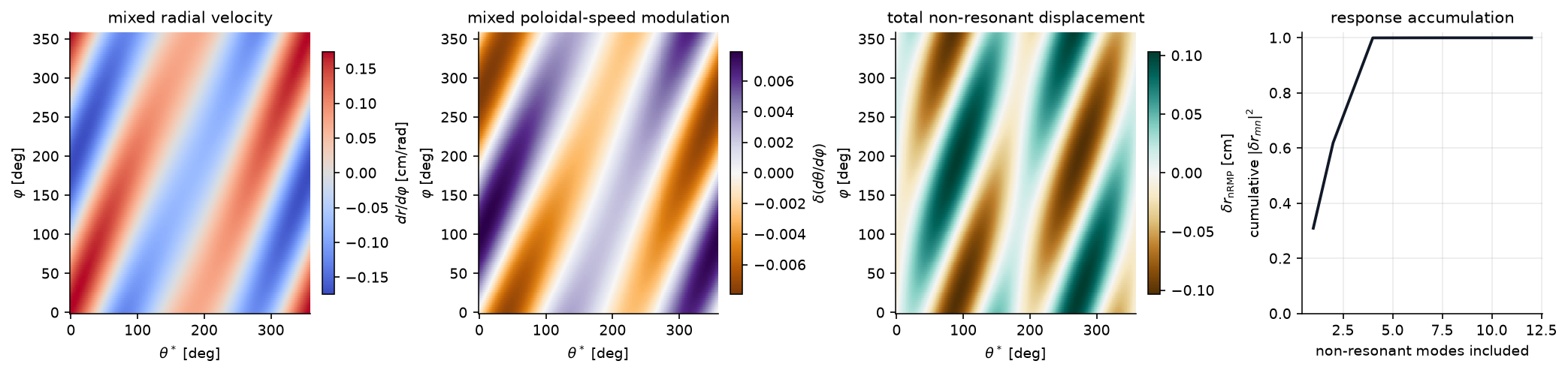
真实扰动很少只包含一个干净的谐波。这个例子把一个共振 (2,1) RMP 与两个非共振分量叠加，其中包括一个 m=1 项。模表会对采样得到的速度谱进行分类，但它只是诊断。计算中的 nRMP 部分是总响应对象：它在绘制平滑位移和速度调制之前，对每个非共振模行求和。

[10]:

mixed_delta_B = compose_magnetic_perturbations(
    delta_B_RMP,
    radial_rmp_field_template(3, 1, amplitude=2.0e-4, phase=0.20, axis_R=eq.R0),
    radial_rmp_field_template(1, 1, amplitude=1.5e-4, phase=0.40, axis_R=eq.R0),
)

mixed_velocity = fieldline_velocity_spectrum_on_circular_surface(
    eq,
    mixed_delta_B,
    psi_res_21,
    n_theta=160,
    n_phi=128,
    m_max=5,
    n_max=4,
    min_amplitude=1e-13,
)
mixed_rows = rmp_nrmp_mode_rows(
    mixed_velocity.radial_spectrum,
    mixed_velocity.iota,
    resonance_tol=1e-10,
    top=12,
    min_amplitude=1e-8,
)
mixed_response = mixed_velocity.nonresonant_response(include_shear=True, resonance_tol=1e-10)

print(f'Local iota on q=2 surface: {mixed_velocity.iota:.6f}')
print(
    'Total nRMP response uses '
    f'{mixed_response.n_nonresonant_modes} non-resonant modes; '
    f'{mixed_response.n_resonant_modes} resonant modes are left for island analysis.'
)
print()
print('RMP/nRMP mode classification diagnostic:')
print('{:<5} {:>8} {:>12} {:>12} {:>12}'.format('kind', '(m,n)', 'detuning', '|F_r mn|', 'phase [deg]'))
print('-' * 56)
for row in mixed_rows:
    print('{:<5} ({:>2d},{:>2d}) {:>12.3e} {:>12.3e} {:>12.2f}'.format(
        row.kind,
        row.m,
        row.n,
        row.detuning,
        row.amplitude,
        row.phase_deg,
    ))

print()
print('Largest contributors to the total nRMP radial response:')
print('{:>8} {:>12} {:>14} {:>14}'.format('(m,n)', 'detuning', '|delta_r_mn| cm', 'cum frac'))
for contrib in mixed_response.contribution_rows(top=8):
    print('({:>2d},{:>2d}) {:>12.3e} {:>14.4f} {:>14.3f}'.format(
        contrib.m,
        contrib.n,
        contrib.detuning,
        100.0 * contrib.radial_response_weight,
        contrib.cumulative_fraction,
    ))

mixed_deformation = mixed_response.deformation
TT_mix, PP_mix, nonres_dr_mix, nonres_dtheta_mix = mixed_response.real_fields()
counts_mix, cumulative_mix = mixed_response.cumulative_contribution()

theta_deg_mix = np.degrees(mixed_velocity.theta)
phi_deg_mix = np.degrees(mixed_velocity.phi)
fig_mix, axes_mix = plt.subplots(1, 4, figsize=(13.8, 3.2), constrained_layout=True)
panels = [
    (mixed_velocity.radial_velocity * 100.0, r'$dr/d\varphi$ [cm/rad]', 'mixed radial velocity', 'coolwarm'),
    (mixed_velocity.poloidal_velocity, r'$\delta(d\theta/d\varphi)$', 'mixed poloidal-speed modulation', 'PuOr'),
    (nonres_dr_mix * 100.0, r'$\delta r_\mathrm{nRMP}$ [cm]', 'total non-resonant displacement', 'BrBG'),
]
for ax, (data, label, title, cmap) in zip(axes_mix[:3], panels):
    vmax = np.nanmax(np.abs(data))
    im = ax.pcolormesh(
        theta_deg_mix,
        phi_deg_mix,
        data,
        shading='auto',
        cmap=cmap,
        vmin=-vmax,
        vmax=vmax,
    )
    ax.set_xlabel(r'$\theta^*$ [deg]')
    ax.set_ylabel(r'$\varphi$ [deg]')
    ax.set_title(title)
    fig_mix.colorbar(im, ax=ax, label=label, shrink=0.86)
axes_mix[3].plot(counts_mix, cumulative_mix, color='#111827', lw=1.8)
axes_mix[3].set_ylim(0, 1.02)
axes_mix[3].set_xlabel('non-resonant modes included')
axes_mix[3].set_ylabel(r'cumulative $|\delta r_{mn}|^2$')
axes_mix[3].set_title('response accumulation')
axes_mix[3].grid(True, alpha=0.25)
plt.show()

Local iota on q=2 surface: 0.500000
Total nRMP response uses 12 non-resonant modes; 2 resonant modes are left for island analysis.

RMP/nRMP mode classification diagnostic:
kind     (m,n)     detuning     |F_r mn|  phase [deg]
--------------------------------------------------------
RMP   (-2, 1)    0.000e+00    6.087e-04        -0.23
RMP   ( 2,-1)    0.000e+00    6.087e-04         0.23
nRMP  (-3, 1)   -5.000e-01    1.442e-04        -9.53
nRMP  ( 3,-1)    5.000e-01    1.442e-04         9.53
nRMP  (-1, 1)    5.000e-01    1.131e-04       -18.07
nRMP  ( 1,-1)   -5.000e-01    1.131e-04        18.07
nRMP  ( 4,-1)    1.000e+00    5.144e-06        10.91
nRMP  (-4, 1)   -1.000e+00    5.144e-06       -10.91
nRMP  ( 0,-1)   -1.000e+00    3.906e-06        21.49
nRMP  ( 0, 1)    1.000e+00    3.906e-06       -21.49
nRMP  (-5, 1)   -1.500e+00    5.000e-08       -11.46
nRMP  ( 5,-1)    1.500e+00    5.000e-08        11.46

Largest contributors to the total nRMP radial response:
   (m,n)     detuning |delta_r_mn| cm       cum frac
(-3, 1)   -5.000e-01         0.0288          0.310
( 3,-1)    5.000e-01         0.0288          0.619
(-1, 1)    5.000e-01         0.0226          0.809
( 1,-1)   -5.000e-01         0.0226          1.000
( 4,-1)    1.000e+00         0.0005          1.000
(-4, 1)   -1.000e+00         0.0005          1.000
( 0, 1)    1.000e+00         0.0004          1.000
( 0,-1)   -1.000e+00         0.0004          1.000

../../../../_images/notebooks_i18n_zh_tutorials_RMP_resonance_analysis_21_1.png

[ORDER_ANALYSIS] 扰动阶数检查#

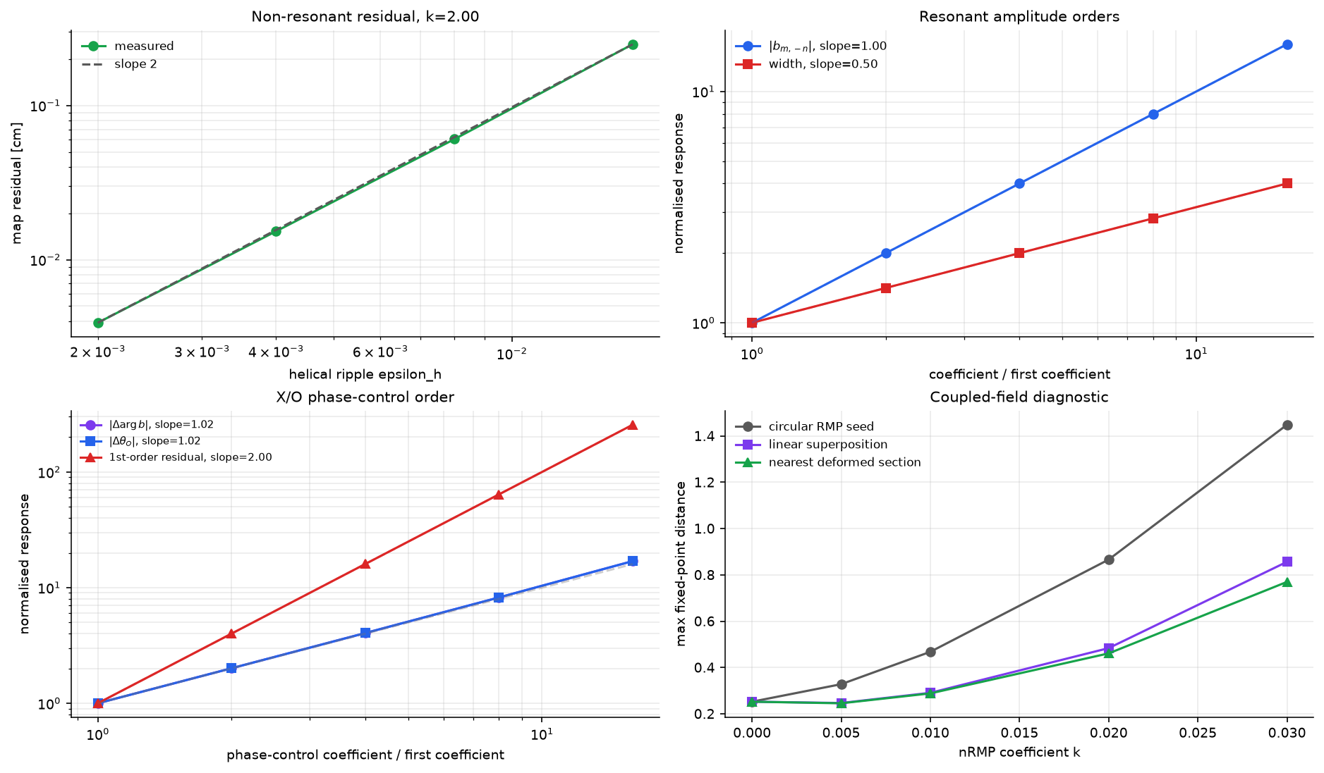
可复用工作流现在集中在几个小型辅助函数中： scan_nonresonant_residual_order, scan_rmp_amplitude_order, scan_rmp_phase_order, scan_rmp_resolution_convergence, 和 plot_perturbation_order_summary。

一旦 Fourier 约定固定，预期阶数就很直接：

nRMP 表面形状残差：一阶形变应留下 O(k^2) 的映射残差。
RMP 共振系数：对 delta B = k f，Fourier 线性给出 |b_{m,-n}| ~ k。
磁岛宽度：Rutherford/Nardon 摆近似宽度按 w ~ sqrt(|b_{m,-n}|) 缩放，因此 w ~ k^{1/2}。
X/O 相位：相位由 arg(b_{m,-n}) 控制，而不是由幅度控制。精确关系为 m*Delta theta_O + Delta arg(b_{m,-n}) = 0。

在相位控制阶数测试中，我们使用无散模板 radial_rmp_field_template。它的相位参数会改变共振系数相位，同时保持 div(delta B)=0，并覆盖重要的 m=1 情形。我们有意测试一个轻微非线性的控制相位 alpha(k)=k+eta*k^2；因此，相对于一阶原始 k 定律的残差应按 O(k^2) 缩放。

[11]:

def component_for_rmp_template(amplitude=1.0e-3, phase=0.0, n_theta=128, n_phi=64):
    return find_resonant_components_analytic(
        eq,
        radial_rmp_field_template(base_m, base_n, amplitude=amplitude, phase=phase, axis_R=eq.R0),
        base_m=base_m,
        base_n=base_n,
        max_harmonic=1,
        n_theta=n_theta,
        n_phi=n_phi,
        min_amplitude=1e-16,
        verbose=False,
    )[0]


def deformed_torus_map_residual(epsilon_h, n_alpha=12):
    eq_case = simple_stellarator(
        R0=eq.R0, r0=eq.r0, B0=eq.B0,
        q0=eq.q0, q1=eq.q1,
        m_h=eq.m_h, n_h=eq.n_h, epsilon_h=float(epsilon_h),
    )
    psi_res = eq_case.resonant_psi(base_m, base_n)[0]
    deformation, r_res, _ = helical_velocity_deformation(
        eq_case, psi_res, n_theta=128, n_phi=128, include_shear=True
    )
    iota = 1.0 / float(eq_case.q_of_psi(psi_res))

    def surface(alpha, phi):
        alpha_arr = np.asarray(alpha)
        return (
            r_res + deformation.section_r(alpha_arr, phi),
            alpha_arr + deformation.section_theta(alpha_arr, phi),
        )

    def rhs(phi, state):
        radius, theta = state
        R = eq_case.R0 + radius*np.cos(theta)
        psi_here = (radius / eq_case.r0)**2
        q_here = float(eq_case.q_of_psi(psi_here))
        Bphi = eq_case.B0 * eq_case.R0 / R
        delta_BR = eq_case.epsilon_h * eq_case.B0 * psi_here * np.cos(eq_case.m_h * theta - eq_case.n_h * phi)
        return [
            R * delta_BR * np.cos(theta) / Bphi,
            1.0/q_here - R * delta_BR * np.sin(theta) / (radius * Bphi),
        ]

    residual = deformed_surface_map_residual(
        surface,
        rhs,
        iota,
        alpha_values=np.linspace(0.0, 2*np.pi, n_alpha, endpoint=False),
        state_to_cartesian=lambda state, phi: [
            eq_case.R0 + float(state[0])*np.cos(float(state[1])),
            float(state[0])*np.sin(float(state[1])),
        ],
    )
    return residual.max_residual


def max_helical_deformation_cm(n_theta, n_phi):
    velocity = fieldline_velocity_spectrum_on_circular_surface(
        eq,
        helical_ripple_delta_B(eq),
        psi_res_21,
        n_theta=max(64, n_theta),
        n_phi=max(64, n_phi),
        m_max=8,
        n_max=8,
        min_amplitude=1e-12,
    )
    deformation = velocity.nonresonant_deformation(include_shear=True)
    TT, PP = np.meshgrid(velocity.theta, velocity.phi, indexing='xy')
    return 100.0 * float(np.nanmax(np.abs(deformation.real_field_r(TT, PP))))


nonres_eps = np.array([0.002, 0.004, 0.008, 0.016])
rmp_k = np.array([2.5e-4, 5e-4, 1e-3, 2e-3, 4e-3])
phase_controls = np.array([0.01, 0.02, 0.04, 0.08, 0.16])
phase_eta = 0.4

nonres_scan = scan_nonresonant_residual_order(nonres_eps, deformed_torus_map_residual)
rmp_amp_scan = scan_rmp_amplitude_order(
    rmp_k,
    lambda k: component_for_rmp_template(amplitude=k, phase=0.0, n_theta=64, n_phi=32),
)
phase_base = component_for_rmp_template(amplitude=1e-3, phase=0.0, n_theta=128, n_phi=64)
phase_scan = scan_rmp_phase_order(
    phase_controls,
    lambda k: component_for_rmp_template(
        amplitude=1e-3,
        phase=float(k) + phase_eta*float(k)*float(k),
        n_theta=128,
        n_phi=64,
    ),
    base_component=phase_base,
)
resolution_scan = scan_rmp_resolution_convergence(
    [(32, 16), (64, 32), (128, 64), (256, 128)],
    lambda n_theta, n_phi: component_for_rmp_template(
        amplitude=1e-3, phase=0.0, n_theta=n_theta, n_phi=n_phi
    ),
    deformation_metric_factory=max_helical_deformation_cm,
)

comp_pos = component_for_rmp_template(amplitude=1e-3, phase=0.0, n_theta=64, n_phi=32)
comp_neg = component_for_rmp_template(amplitude=-1e-3, phase=0.0, n_theta=64, n_phi=32)
sign_phase_jump_deg = float(np.degrees(np.angle(comp_neg.b_mn / comp_pos.b_mn)))

print(f'Non-resonant deformation residual slope = {nonres_scan.slope:.3f} (expected 2)')
print(f'Positive RMP: |b_mn| slope =             {rmp_amp_scan.b_fit.slope:.3f} (expected 1)')
print(f'Positive RMP: island half-width slope =  {rmp_amp_scan.width_fit.slope:.3f} (expected 0.5)')
print(f'Positive RMP: X/O phase span:           {rmp_amp_scan.phase_span_deg:.3e} deg')
print(f'Negative coefficient: arg jump:         {sign_phase_jump_deg:.1f} deg')
print(f'  +k: O={np.degrees(comp_pos.opoint_theta):.1f} deg, X={np.degrees(comp_pos.xpoint_theta):.1f} deg')
print(f'  -k: O={np.degrees(comp_neg.opoint_theta):.1f} deg, X={np.degrees(comp_neg.xpoint_theta):.1f} deg')
print(f'Phase template: |Delta arg b| slope =    {phase_scan.b_phase_fit.slope:.3f} (locally expected 1)')
print(f'Phase template: |Delta theta_O| vs |Delta arg b| slope = {phase_scan.opoint_vs_b_phase_fit.slope:.3f} (expected 1)')
print(f'Phase template: max |m Delta theta_O + Delta arg b|: {phase_scan.max_exact_relation_residual:.3e} rad')
print(f'Phase template: first-order residual slope = {phase_scan.first_order_residual_fit.slope:.3f} (expected 2)')

print()
print('Resolution convergence against the finest RMP spectrum grid:')
print('{:>8} {:>6} {:>12} {:>14} {:>14} {:>14}'.format(
    'n_theta', 'n_phi', 'rel |b| err', 'phase err deg', 'rel width err', 'max |dr| cm'
))
for row in resolution_scan.rows:
    print(f'{row.n_theta:8d} {row.n_phi:6d} {row.relative_b_error:12.3e} '
          f'{row.phase_error_deg:14.3e} {row.relative_width_error:14.3e} '
          f'{row.deformation_metric:14.4f}')

coupling_sweep = None
if components:
    component = components[0]

    def coupled_distances(eps_h):
        eq_case = simple_stellarator(
            R0=eq.R0, r0=eq.r0, B0=eq.B0,
            q0=eq.q0, q1=eq.q1,
            m_h=eq.m_h, n_h=eq.n_h, epsilon_h=float(eps_h),
        )
        rows = compare_cyna_fixed_points_for_component(
            sample_stellarator_cylindrical_field(
                eq_case, delta_B_RMP, nR=128, nPhi=128, label=f'coupled_rmp_eps_{eps_h:.3f}',
            ),
            component,
            eq_case,
            DPhi=0.015,
            max_iter=80,
            tol=1e-11,
            n_threads=4,
        )
        raw_cm = max(np.hypot(row.newton_R - row.predicted_R, row.newton_Z - row.predicted_Z) for row in rows) * 100.0
        if eps_h == 0.0:
            return raw_cm, raw_cm, raw_cm
        deformation, r_res, _ = helical_velocity_deformation(eq_case, component.psi_res, include_shear=True)
        superposed_cm = max(
            np.hypot(
                float(deformed_circular_section_rz(eq_case, r_res, deformation, row.predicted_theta)[0]) - row.newton_R,
                float(deformed_circular_section_rz(eq_case, r_res, deformation, row.predicted_theta)[1]) - row.newton_Z,
            ) for row in rows
        ) * 100.0
        projected = project_fixed_points_to_deformed_surface(rows, eq_case, deformation, r_minor=r_res)
        return raw_cm, superposed_cm, max(row.distance_cm for row in projected)

    try:
        coupling_sweep = scan_coupled_fixed_point_sweep(np.array([0.0, 0.005, 0.01, 0.02, 0.03]), coupled_distances)
    except ImportError as exc:
        print('Coupled cyna sweep skipped:', exc)

if coupling_sweep is not None:
    print()
    print('Coupled RMP + helical ripple, fixed RMP amplitude:')
    print('{:>9} {:>12} {:>16} {:>16}'.format('epsilon_h', 'raw [cm]', 'superposed [cm]', 'nearest [cm]'))
    for eps_h, raw_cm, superposed_cm, nearest_cm in zip(
        coupling_sweep.k, coupling_sweep.raw_distance,
        coupling_sweep.superposed_distance, coupling_sweep.nearest_deformed_distance,
    ):
        print(f'{eps_h:9.3f} {raw_cm:12.4f} {superposed_cm:16.4f} {nearest_cm:16.4f}')

fig_order, axes_order = plot_perturbation_order_summary(
    nonresonant=nonres_scan,
    rmp_amplitude=rmp_amp_scan,
    rmp_phase=phase_scan,
    coupling=coupling_sweep,
    residual_scale=100.0,
    residual_label='map residual [cm]',
    coefficient_label='helical ripple epsilon_h',
)
plt.show()

Non-resonant deformation residual slope = 1.999 (expected 2)
Positive RMP: |b_mn| slope =             1.000 (expected 1)
Positive RMP: island half-width slope =  0.500 (expected 0.5)
Positive RMP: X/O phase span:           0.000e+00 deg
Negative coefficient: arg jump:         180.0 deg
  +k: O=135.0 deg, X=45.0 deg
  -k: O=45.0 deg, X=135.0 deg
Phase template: |Delta arg b| slope =    1.020 (locally expected 1)
Phase template: |Delta theta_O| vs |Delta arg b| slope = 1.000 (expected 1)
Phase template: max |m Delta theta_O + Delta arg b|: 4.441e-16 rad
Phase template: first-order residual slope = 2.000 (expected 2)

Resolution convergence against the finest RMP spectrum grid:
 n_theta  n_phi  rel |b| err  phase err deg  rel width err    max |dr| cm
      32     16    0.000e+00      0.000e+00      0.000e+00         1.2408
      64     32    0.000e+00      0.000e+00      0.000e+00         1.2408
     128     64    0.000e+00      0.000e+00      0.000e+00         1.2408
     256    128    0.000e+00      0.000e+00      0.000e+00         1.2408

Coupled RMP + helical ripple, fixed RMP amplitude:
epsilon_h     raw [cm]  superposed [cm]     nearest [cm]
    0.000       0.2524           0.2524           0.2524
    0.005       0.3280           0.2467           0.2455
    0.010       0.4678           0.2908           0.2883
    0.020       0.8661           0.4838           0.4610
    0.030       1.4484           0.8564           0.7698

../../../../_images/notebooks_i18n_zh_tutorials_RMP_resonance_analysis_23_1.png

[ISLAND_WIDTHS] 磁岛宽度柱状图与 Chirikov 重叠图#

Chirikov 重叠参数定义为

\[\sigma = \frac{w_1 + w_2}{|r_1 - r_2|}\]

其中 \(w_i\) 是半宽，\(r_i\) 是相邻磁岛的径向位置。当 \(\sigma \gtrsim 1\) 时，随机输运开始出现。

[12]:

fig_iw, (ax_bar, ax_q) = plt.subplots(1, 2, figsize=(9, 3.8))

# ── (a) Island width bar chart ───────────────────────────────────────────
labels = [f'$({c.m},{c.n})$\nq={c.q_res:.2f}' for c in components]
widths_cm = [c.half_width_r * 100 for c in components]
colors_bar = [ISLAND_CMAPS[(c.harmonic_order - 1) % len(ISLAND_CMAPS)] for c in components]

x_pos = np.arange(len(components))
bars = ax_bar.bar(x_pos, widths_cm, color=colors_bar, edgecolor='k',
                  linewidth=0.7, alpha=0.85, width=0.55)
for bar, w in zip(bars, widths_cm):
    ax_bar.text(bar.get_x() + bar.get_width()/2, w + 0.05,
                f'{w:.2f}', ha='center', va='bottom', fontsize=8)

ax_bar.set_xticks(x_pos)
ax_bar.set_xticklabels(labels, fontsize=8)
ax_bar.set_ylabel('Island half-width (cm)')
ax_bar.set_title('Island Width by Harmonic')
ax_bar.set_ylim(0, max(widths_cm)*1.25 if widths_cm else 1)

# ── (b) q-profile with island width bands ───────────────────────────────
psi_arr = np.linspace(0, 1, 200)
r_arr = np.sqrt(psi_arr) * eq.r0
q_arr = eq.q_of_psi(psi_arr)

ax_q.plot(r_arr * 100, q_arr, 'k-', linewidth=1.5, label='q(r)')
ax_q.set_xlabel('r (cm)')
ax_q.set_ylabel('Safety factor q')
ax_q.set_title('q-profile with Island Width Bands')

# Draw horizontal bands for each resonance
chirikov_pairs = []
for c in components:
    color = ISLAND_CMAPS[(c.harmonic_order - 1) % len(ISLAND_CMAPS)]
    r_res = np.sqrt(c.psi_res) * eq.r0 * 100  # cm
    w_r = c.half_width_r * 100  # cm
    q_res = c.q_res
    # Island band in r
    ax_q.axvspan(r_res - w_r, r_res + w_r, alpha=0.25, color=color, zorder=2)
    ax_q.axhline(q_res, color=color, lw=0.8, linestyle='--', alpha=0.7)
    ax_q.text(r_res + w_r + 0.2, q_res, f'$({c.m},{c.n})$',
              color=color, fontsize=8, va='center')
    chirikov_pairs.append((r_res, w_r))

# Chirikov overlap
if len(chirikov_pairs) >= 2:
    for i in range(len(chirikov_pairs) - 1):
        r1, w1 = chirikov_pairs[i]
        r2, w2 = chirikov_pairs[i+1]
        gap = abs(r2 - r1)
        sigma = (w1 + w2) / gap if gap > 0 else float('inf')
        print(f'Chirikov sigma between ({components[i].m},{components[i].n}) and ({components[i+1].m},{components[i+1].n}): {sigma:.3f}')

ax_q.set_xlim(0, eq.r0 * 100 * 1.05)
ax_q.grid(True, alpha=0.3)

plt.tight_layout()
plt.show()

../../../../_images/notebooks_i18n_zh_tutorials_RMP_resonance_analysis_25_0.png

[MN_SPECTRUM] 二维 Fourier 谱热图#

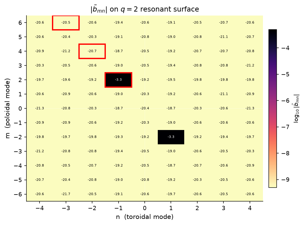
我们在主共振面上计算无散度 RMP 模板的完整 \((m,n)\) Fourier 谱。图中高亮共振模 \((2,-1)\) 及其被驱动的谐波；上面的混合谱截面则是配套视图，它按失谐量对共振模行和非共振模行进行分类。

[13]:

psi_res_21 = eq.resonant_psi(2, 1)[0]
print(f'Computing (m,n) spectrum on q=2 surface (psi={psi_res_21:.3f}), n_theta=48, n_phi=48...')
b_mn = compute_mn_spectrum(
    delta_B_RMP,
    S=psi_res_21,
    equilibrium=eq,
    m_max=6,
    n_max=4,
    n_theta=48,
    n_phi=48,
)
print(f'Spectrum shape: {b_mn.shape}')

fig_sp, ax_sp = plt.subplots(figsize=(7, 5))
plot_mn_heatmap(
    b_mn, m_max=6, n_max=4,
    ax=ax_sp,
    log_scale=True,
    title=r'$|\tilde{b}_{mn}|$ on $q=2$ resonant surface',
    cmap='magma_r',
    highlight_modes=[(2, -1), (4, -2), (6, -3)],
)
plt.tight_layout()
plt.show()

Computing (m,n) spectrum on q=2 surface (psi=0.167), n_theta=48, n_phi=48...
Spectrum shape: (13, 9)

../../../../_images/notebooks_i18n_zh_tutorials_RMP_resonance_analysis_27_1.png

[MAGNETIC_SPECTRUM_ATLAS] 多分量逆变 \(B^r\) 谱图册#

上面的单面热图有助于检查主导 RMP 模行，但生产级磁拓扑分析通常需要谱族视图。这里我们构造一个无散度的多分量扰动，在径向堆栈上计算 Nardon 规范的逆变径向谱 \(\tilde b^1_{mn}=\delta B^1/B_0^3\)，并一起分析所有请求的共振模行。

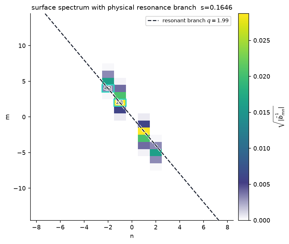
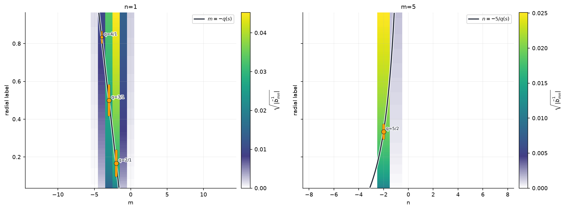
下面的工具有意保持模块化。显示的图册使用更宽的带符号 Fourier 窗口、97 个径向面、amplitude_scale='sqrt'，并用白色遮罩表示零值/缺失模行。非对数 colormap 也从同一个白色基线开始，因此接近零的系数不会看起来与遮罩背景人为分离。带符号坐标轴显示计算谱中的实际 Fourier 模行：对于实场，(m,n) 与 (-m,-n) 共轭，但除非扰动模型施加额外对称性，否则 (m,n) 与 (m,-n) 是独立的相反螺旋度模行。当目标是严格审计动态范围而不是识别视觉模式时，amplitude_scale='log10' 仍然有用。

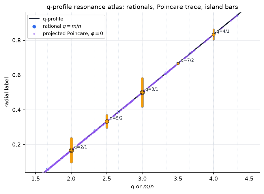
plot_rational_surface_map 在 (m/n, s) 平面中组合可选的 q 剖面、低阶有理面标记、投影 Poincaré 点和磁岛宽度条。
plot_spectrum_heatmap(..., renderer='pcolormesh') 是推荐的表面谱视图；它可以叠加物理共振分支 m=-q n_F，而不绘制相反螺旋度分支。
plot_spectrum_bar3d 返回可交互的 Plotly 图，用于旋转、缩放和悬停检查主导行。
plot_radial_mode_heatmap(fixed_n=..., resonant_sign=+1) 跟踪固定 Fourier \(n\) 下的所有 \(m\) 模行，并在负 \(m\) 半平面绘制正 q 分支 \(m=-nq(s)\)。
plot_radial_mode_heatmap(fixed_m=..., axis_convention='fourier') 跟踪实际 Fourier \(n\) 模行，并绘制正 q 分支 \(n=-m/q(s)\)；q 曲线和磁岛宽度条仍可独立开关。

黄色竖条标记低阶有理面上的单系数 Nardon 半宽估计；其厚度随共振系数幅度缩放。它们是可选叠加层，不属于热图本身。每个径向图只绘制物理共振曲线。相反螺旋度分支不是共轭诊断，因此这里有意不镜像绘制。如果多个谐波共享同一个约化有理面，真实的有限幅度磁岛宽度应从组合后的共振 Hamiltonian 计算；逐行竖条只是诊断，而不是那个非线性求和宽度。

[14]:

delta_B_multi_rmp = compose_magnetic_perturbations(
    radial_rmp_field_template(2, 1, amplitude=5.0e-4, phase=0.00, axis_R=eq.R0),
    radial_rmp_field_template(3, 1, amplitude=2.4e-4, phase=0.55, axis_R=eq.R0),
    radial_rmp_field_template(5, 2, amplitude=1.6e-4, phase=-0.35, axis_R=eq.R0),
)

S_scan = np.linspace(0.04, 0.96, 97)
theta_spec = np.linspace(0.0, 2*np.pi, 160, endpoint=False)
phi_spec = np.linspace(0.0, 2*np.pi, 96, endpoint=False)

theta_grid = theta_spec[None, None, :]
phi_grid = phi_spec[:, None, None]
r_scan = eq.r0 * np.sqrt(S_scan)[None, :, None]
R_stack = eq.R0 + r_scan * np.cos(theta_grid)
Z_stack = r_scan * np.sin(theta_grid)
R_stack = np.repeat(R_stack, phi_spec.size, axis=0)
Z_stack = np.repeat(Z_stack, phi_spec.size, axis=0)
Phi_stack = phi_grid + np.zeros_like(R_stack)

dBR_stack, dBZ_stack, dBphi_stack = delta_B_multi_rmp(R_stack, Z_stack, Phi_stack)
Bphi0_stack = eq.B0 * eq.R0 / np.maximum(R_stack, 1.0e-12)
tilde_b1_grid = nardon_radial_perturbation(
    R_stack,
    Z_stack,
    phi_spec,
    theta_spec,
    dBR_stack,
    dBZ_stack,
    dBphi_stack,
    S_scan,
    denominator_B_phi=Bphi0_stack,
)
magnetic_spectrum = radial_perturbation_Fourier_spectrum(
    tilde_b1_grid,
    theta_spec,
    phi_spec,
    radial_labels=S_scan,
    m_max=14,
    n_max=8,
    min_amplitude=1.0e-14,
)
q_scan = eq.q_of_psi(S_scan)
n_scan = [1, 2, 3]
m_scan = {1: range(1, 9), 2: range(2, 13), 3: range(3, 15)}
chains_multi = analyze_resonant_island_chains_multi_n(
    magnetic_spectrum,
    q_scan,
    n_values=n_scan,
    m_values=m_scan,
    min_b_res=1.0e-8,
)

print(f'Radial spectrum: {S_scan.size} surfaces, {magnetic_spectrum.m.size} retained Fourier rows over |m|<=14, |n|<=8.')
print(f'Multi-RMP analysis found {len(chains_multi)} resonant island-chain estimates.')
print('{:>7} {:>9} {:>9} {:>12} {:>12} {:>10}'.format('(m,n)', 's_res', 'q_res', 'b_res', 'half_width', 'phase'))
for chain in sorted(chains_multi, key=lambda item: item.b_res, reverse=True)[:8]:
    print('({:>2d},{:>1d}) {:>9.4f} {:>9.4f} {:>12.3e} {:>12.3e} {:>9.1f}°'.format(
        chain.m, chain.n, chain.radial_label, chain.q, chain.b_res, chain.half_width, np.degrees(chain.phase)
    ))

review_root = PROJECT_ROOT if PROJECT_ROOT is not None else pathlib.Path.cwd()
review_dir = review_root / 'pyna_output/magnetic_spectrum_review'
review_dir.mkdir(parents=True, exist_ok=True)

poincare_trace = None
if 'R_cross_p0' in globals() and len(R_cross_p0):
    S_p0 = np.clip(((R_cross_p0 - eq.R0)**2 + Z_cross_p0**2) / eq.r0**2, 0.0, 1.0)
    q_p0 = eq.q_of_psi(S_p0)
    poincare_trace = PoincareRationalTrace(
        ratio=q_p0,
        radial_label=S_p0,
        label=r'projected Poincare, $\varphi=0$',
    )

fig_qmap, ax_qmap, rational_markers = plot_rational_surface_map(
    S_scan,
    q_scan,
    n_values=n_scan,
    m_values=m_scan,
    chains=chains_multi,
    poincare=poincare_trace,
    show_poincare=poincare_trace is not None,
    max_island_bars=12,
    annotate_rationals=False,
    title='q-profile resonance atlas: rationals, Poincare trace, island bars',
)
fig_qmap.savefig(review_dir / '01_q_profile_resonance_map.png', dpi=180, bbox_inches='tight', facecolor='white')
plt.show()

surface_index = int(np.argmin(np.abs(S_scan - psi_res_21)))
surface_label = float(S_scan[surface_index])
chains_surface = [chain for chain in chains_multi if abs(chain.radial_label - surface_label) <= 0.08]
fig_surface, ax_surface = plt.subplots(figsize=(6.7, 5.7))
plot_spectrum_heatmap(
    magnetic_spectrum,
    radial_index=surface_index,
    m_values=np.arange(-14, 15),
    n_values=np.arange(-8, 9),
    chains=chains_surface,
    q_value=float(q_scan[surface_index]),
    renderer='pcolormesh',
    amplitude_scale='sqrt',
    mask_zeros=True,
    ax=ax_surface,
    cmap='viridis',
    title='surface spectrum with physical resonance branch',
)
fig_surface.savefig(review_dir / '02_surface_pcolormesh_atlas.png', dpi=180, bbox_inches='tight', facecolor='white')
plt.show()

fig_bar3d = plot_spectrum_bar3d(
    magnetic_spectrum,
    radial_index=surface_index,
    m_values=np.arange(-10, 11),
    n_values=np.arange(-6, 7),
    amplitude_scale='sqrt',
    range_mode='nonzero',
    bar_width=0.9,
    z_aspect=0.72,
    title='interactive 3D spectrum bars',
)
fig_bar3d.write_html(str(review_dir / '04_surface_plotly_bar3d.html'), include_plotlyjs='cdn')
try:
    fig_bar3d.write_image(str(review_dir / '04_surface_plotly_bar3d.png'), width=1040, height=650, scale=2)
except Exception as exc:
    print(f'Plotly static PNG export skipped: {exc}')
fig_bar3d.show()

fig_radial, axes_radial = plt.subplots(1, 2, figsize=(13.2, 4.9), sharey=True)
plot_radial_mode_heatmap(
    magnetic_spectrum,
    fixed_n=1,
    mode_values=np.arange(-14, 15),
    resonant_sign=1,
    q_profile=q_scan,
    chains=chains_multi,
    renderer='pcolormesh',
    amplitude_scale='sqrt',
    mask_zeros=True,
    ax=axes_radial[0],
    cmap='viridis',
    title='n=1',
)
plot_radial_mode_heatmap(
    magnetic_spectrum,
    fixed_m=5,
    mode_values=np.arange(-8, 9),
    axis_convention='fourier',
    q_profile=q_scan,
    chains=chains_multi,
    renderer='pcolormesh',
    amplitude_scale='sqrt',
    mask_zeros=True,
    ax=axes_radial[1],
    cmap='viridis',
    title='m=5',
)
plt.tight_layout()
fig_radial.savefig(review_dir / '03_radial_fixed_n_fixed_m_maps.png', dpi=180, bbox_inches='tight', facecolor='white')
plt.show()

Radial spectrum: 97 surfaces, 22 retained Fourier rows over |m|<=14, |n|<=8.
Multi-RMP analysis found 7 resonant island-chain estimates.
  (m,n)     s_res     q_res        b_res   half_width      phase
( 2,1)    0.1667    2.0000    1.661e-03    6.655e-02       0.6°
( 3,1)    0.5000    3.0000    1.535e-03    7.836e-02      27.6°
( 5,2)    0.3333    2.5000    7.401e-04    3.512e-02     -20.1°
( 4,1)    0.8333    4.0000    1.665e-04    2.980e-02      30.1°
( 6,2)    0.5000    3.0000    6.400e-05    1.131e-02     -20.1°
( 4,2)    0.1667    2.0000    2.132e-05    5.332e-03     -20.1°
( 7,2)    0.6667    3.5000    1.742e-06    2.016e-03     -20.1°

../../../../_images/notebooks_i18n_zh_tutorials_RMP_resonance_analysis_29_1.png

../../../../_images/notebooks_i18n_zh_tutorials_RMP_resonance_analysis_29_2.png

Data type cannot be displayed: application/vnd.plotly.v1+json

../../../../_images/notebooks_i18n_zh_tutorials_RMP_resonance_analysis_29_4.png

[PUBLICATION_FIGURE] 多环向角六面板图#

同一个截面辅助函数可以扩展到紧凑的多截面布局。O/X 标记、O 点磁岛宽度条和局部稳定分支会随环向角旋转，而 PEST 风格网格让每个面板中的坐标含义保持可见。

[15]:

fig_pub, axes_pub = plot_rmp_resonance_sections(
    all_sections_data,
    phi_sections,
    eq=eq,
    components=components,
    colors=ISLAND_CMAPS,
    ncols=3,
    figsize=(12.0, 7.0),
    point_size=1.6,
    point_alpha=0.42,
    compact=True,
    overlays=('pest_grid', 'poincare', 'resonant_surfaces', 'stable_branches', 'island_width_bars', 'xo'),
    title=(
        'Stellarator RMP resonance: Poincare points, X/O geometry, '
        'island-width bars, stable branches, and PEST-style grid'
    ),
)

out_path = pathlib.Path('pyna_output/rmp_resonance_publication.png')
out_path.parent.mkdir(exist_ok=True)
fig_pub.savefig(str(out_path), dpi=170, bbox_inches='tight', facecolor='white')
print(f'Saved publication figure to {out_path}')
from IPython.display import display
display(fig_pub)
plt.close(fig_pub)

Saved publication figure to pyna_output/rmp_resonance_publication.png

../../../../_images/notebooks_i18n_zh_tutorials_RMP_resonance_analysis_31_1.png