RMP-Stellarator-Resonanzanalyse#
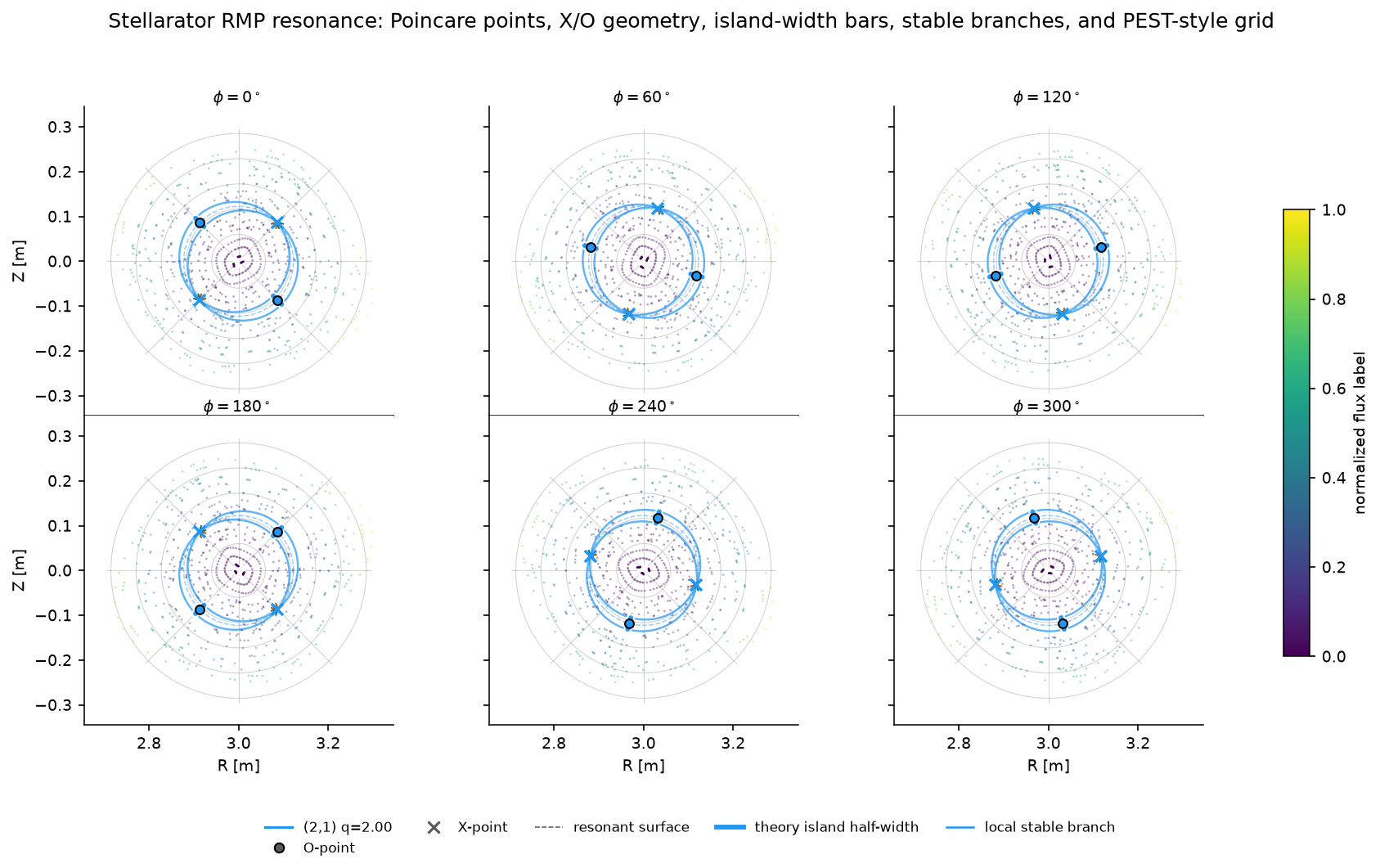
Dieses Notebook ist der zentrale öffentliche Workflow für analytische Stellarator-Resonanzgeometrie. Es führt zwei früher getrennte, rein textuelle Tutorials zu einer visuellen Berechnung zusammen:
Ein analytisches Stellarator-Gleichgewicht aufbauen und Poincaré-Schnitte verfolgen.
Resonante RMP-Fourier-Komponenten und ihre analytischen X/O-Fixpunkte berechnen.
Rohe Schnittpunkte zu Geometrie hochstufen: Kreuzungen, Fixpunktmarker, resonante Flächen, O-Punkt-Inselbreitenbalken, lokale stabile Äste und Koordinaten-Overlays.
Ungestörte und gestörte Schnitte mit einem PEST-artigen Gitter vergleichen.
Inselbreiten, Chirikov-Überlappung und das \((m,n)\)-Spektrum zusammenfassen.
Mit
pyna.plot-Hilfsfunktionen eine moderne Mehrschnitt-Abbildung erzeugen.
Das Notebook ist dafür vorgesehen, lokal vor der Veröffentlichung der Dokumentation ausgeführt zu werden. GitHub Pages rendert die gespeicherten Ausgaben, statt Feldlinienverfolgungen neu zu berechnen.
[SETUP] Importe und Publikationsstil#
[1]:
import sys
import json
import pathlib
import numpy as np
import matplotlib
import matplotlib.pyplot as plt
from matplotlib.colors import Normalize

PROJECT_ROOT = None
for candidate in [pathlib.Path.cwd(), *pathlib.Path.cwd().parents]:
    if (candidate / 'pyna').is_dir() and (candidate / 'pyproject.toml').exists():
        PROJECT_ROOT = candidate
        break
if PROJECT_ROOT is not None and str(PROJECT_ROOT) not in sys.path:
    sys.path.insert(0, str(PROJECT_ROOT))

%matplotlib inline
from matplotlib_inline.backend_inline import set_matplotlib_formats
set_matplotlib_formats('png')

plt.rcParams.update({
    'font.family': 'DejaVu Sans',
    'font.size': 9,
    'axes.labelsize': 9,
    'axes.titlesize': 10,
    'figure.dpi': 150,
    'text.usetex': False,
    'axes.linewidth': 0.75,
    'axes.spines.top': False,
    'axes.spines.right': False,
    'figure.facecolor': 'white',
    'axes.facecolor': 'white',
})

from pyna.toroidal.equilibrium.stellarator import simple_stellarator
from pyna.toroidal.visual.RMP_spectrum import (
    find_resonant_components_analytic,
    radial_rmp_field_template,
    compose_magnetic_perturbations,
    circular_shell_divergence_diagnostic,
    fieldline_velocity_spectrum_on_circular_surface,
    rmp_nrmp_Modus_rows,
    sample_stellarator_cylindrical_field,
    compare_cyna_fixed_points_for_component,
    deformed_circular_section_rz,
    deformed_surface_map_residual,
    project_fixed_points_to_deformed_surface,
    CoupledFixedPointSweep,
    plot_perturbation_order_summary,
    scan_nonresonant_residual_order,
    scan_coupled_fixed_point_sweep,
    scan_rmp_amplitude_order,
    scan_rmp_phase_order,
    scan_rmp_resolution_convergence,
    compute_mn_spectrum,
    plot_mn_heatmap,
    ISLAND_CMAPS,
)
from pyna.toroidal.perturbation_spectrum import (
    analyze_resonant_island_chains_multi_n,
    nardon_radial_perturbation,
    radial_perturbation_Fourier_spectrum,
)
from pyna.toroidal.visual.magnetic_spectrum import (
    PoincaréRationalTrace,
    plot_radial_Modus_heatmap,
    plot_rational_surface_map,
    plot_spectrum_bar3d,
    plot_spectrum_heatmap,
)
from pyna.topo.poincare import poincare_from_fieldlines, ToroidalSection
from pyna.plot import (
    draw_pest_grid,
    draw_poincare_points,
    draw_rmp_resonance_section,
    plot_rmp_resonance_sections,
)

print('Einrichtung abgeschlossen. numpy', np.__version__, '  matplotlib', matplotlib.__version__)
Einrichtung abgeschlossen. numpy 2.4.6 matplotlib 3.11.0
[EQ] Stellarator-Gleichgewicht aufbauen#
Wir verwenden einen analytischen Stellarator mit einzelner Helizität:
Großer Radius \(R_0 = 3.0\) m, kleiner Radius \(r_0 = 0.3\) m, Achsenfeld \(B_0 = 2.5\) T
Lineares \(q\)-Profil: \(q_0=1.5\) (Achse) bis \(q_1=4.5\) (LCFS)
Helikales Ripple: \((m_h, n_h) = (3,3)\), \(\epsilon_h = 0.03\)
Das Sicherheitsfaktorprofil \(q(\psi) = q_0 + (q_1-q_0)\psi\) spannt den Bereich \([1.5, 4.5]\) auf, sodass Resonanzen bei \(q = 2/1, 3/1, 4/1\) und weitere im Plasma liegen.
[2]:
eq = simple_stellarator(
    R0=3.0, r0=0.3, B0=2.5,
    q0=1.5, q1=4.5,
    m_h=3, n_h=3, epsilon_h=0.03,
)
print(eq)
print(f'q-Bereich: [{eq.q0}, {eq.q1}]')
print(f'Resonanzfläche für (2,1): psi_res = {eq.resonant_psi(2,1)}')
print(f'Resonanzfläche für (4,2): psi_res = {eq.resonant_psi(4,2)}')
print(f'Resonanzfläche für (6,3): psi_res = {eq.resonant_psi(6,3)}')

# Convenience references
R0_eq = eq.R0
r0_eq = eq.r0
StellaratorSimple(R0=3.0 m, r0=0.3 m, B0=2.5 T, q=[1.5, 4.5], m_h=3, n_h=3, ε_h=0.03)
q-Bereich: [1.5, 4.5]
Resonanzfläche für (2,1): psi_res = [0.16666666666666666]
Resonanzfläche für (4,2): psi_res = [0.16666666666666666]
Resonanzfläche für (6,3): psi_res = [0.16666666666666666]
[RMP_NRMP_WORKFLOW] RMP/nRMP-Zerlegung#
Ein Störungsmodus auf einer Flussfläche ist erst dann nützlich, wenn er mit der lokalen Feldlinienrotation verglichen wird. Mit der Fourier-Konvention
ist die lokale Verstimmung
Teil |
Bedingung |
geometrischer Effekt |
pyna-Workflow |
|---|---|---|---|
RMP |
|
öffnet Inselketten; X/O-Punkte, O-Punkt-Breitenbalken und Separatrix-Äste sind sinnvolle Objekte erster Ordnung |
|
nRMP |
|
alle nichtresonanten Moden tragen zu glatter Flussflächenverformung und Feldlinien-Geschwindigkeitsmodulation bei |
|
gemischtes Spektrum |
beides vorhanden |
resonante Inselgeometrie liegt auf der insgesamt nRMP-verformten Fläche |
|
Validierung |
Vektorfeld muss physikalisch sein |
ein nicht-solenoidales Template kann falsche Topologie erzeugen |
|
Der zentrale Unterschied: Eine RMP-Diagnostik fokussiert resonante Zeilen, während eine nRMP-Antwort die vollständige Summe über alle nichtresonanten Zeilen ist:
Beitragstabellen sind für Rangordnung und Konvergenz nützlich; das Modell ist aber das vollständige nichtresonante Spektrum, nicht eine ausgewählte Spitzenkomponente.
[POINCARE_UNPERTURBED] Ungestörter Poincaré-Schnitt bei phi=0#
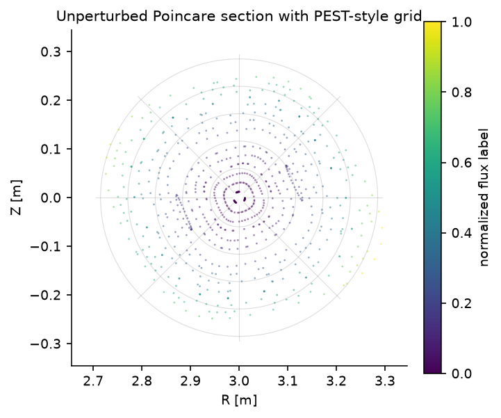
Wir verfolgen Feldlinien des ungestörten Gleichgewichts und zeichnen Kreuzungen mit der \(\varphi=0\)-Ebene auf. Das Ergebnis ist die rohe abgetastete Geometrie: nützlich, aber noch kein topologisches Objekt. Spätere Zellen fügen die Hochstufungsschicht hinzu, indem resonante Flächen, X/O-Marker, lokale stabile Äste und ein PEST-artiges Koordinatengitter überlagert werden.
Kreuzungen werden in pyna_output/poincare_unperturbed.json zwischengespeichert.
[3]:
CACHE_UNPERT = pathlib.Path('pyna_output/poincare_unperturbed.json')
CACHE_UNPERT.parent.mkdir(exist_ok=True)

if CACHE_UNPERT.exists():
    _d = json.loads(CACHE_UNPERT.read_text())
    R_cross_u = np.array(_d['R'])
    Z_cross_u = np.array(_d['Z'])
    print(f'Aus Cache geladen: {len(R_cross_u)} Kreuzungen')
else:
    n_fieldlines = 15
    n_turns = 50
    dt = 0.08
    t_max = n_turns * 2 * np.pi * eq.R0

    R_starts = np.linspace(eq.R0 + 0.04*eq.r0, eq.R0 + 0.92*eq.r0, n_fieldlines)
    start_pts = np.zeros((n_fieldlines, 3))
    start_pts[:, 0] = R_starts
    start_pts[:, 2] = 0.0

    sections_u = [ToroidalSection(phi0=0.0)]
    print(f'Verfolge {n_fieldlines} Feldlinien x {n_turns} Umläufe (dt={dt}, t_max={t_max:.1f} m)...')

    pmap_u = poincare_from_fieldlines(
        eq.field_func,
        start_pts,
        sections_u,
        t_max=t_max,
        dt=dt,
    )
    arr_u = pmap_u.crossing_array(0)
    R_cross_u = arr_u[:, 0]
    Z_cross_u = arr_u[:, 1]
    print(f'Berechnet: {len(R_cross_u)} Kreuzungen. Zwischenspeichern...')
    CACHE_UNPERT.write_text(json.dumps({'R': R_cross_u.tolist(), 'Z': Z_cross_u.tolist()}))
    print('Zwischengespeichert.')

fig_u, ax_u = plt.subplots(figsize=(4.7, 4.3), constrained_layout=True)
draw_pest_grid(ax_u, eq, alpha=0.22)
psi_pts = np.clip(((R_cross_u - eq.R0)**2 + Z_cross_u**2) / eq.r0**2, 0, 1)
draw_poincare_points(
    ax_u,
    R_cross_u,
    Z_cross_u,
    values=psi_pts,
    cmap='viridis',
    point_size=1.8,
    alpha=0.50,
    rasterized=False,
)
sm_u = plt.cm.ScalarMappable(cmap='viridis', norm=Normalize(0, 1))
fig_u.colorbar(sm_u, ax=ax_u, label='normalized flux label', shrink=0.82)
lim = 1.15 * eq.r0
ax_u.set_xlim(eq.R0 - lim, eq.R0 + lim)
ax_u.set_ylim(-lim, lim)
ax_u.set_aspect('equal')
ax_u.set_xlabel('R [m]')
ax_u.set_ylabel('Z [m]')
ax_u.set_title('Unperturbed Poincaré section with PEST-style grid')
plt.show()
Aus Cache geladen: 735 Kreuzungen
[RMP_FIELD] RMP-Störfeld definieren und visualisieren#
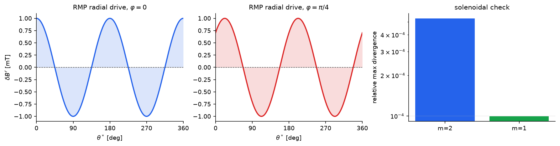
Wir verwenden eine einmodige RMP mit Basismodus \((m,n)=(2,1)\) und Amplitude \(\delta B=1\) mT. Das nutzerseitige Template lautet
aber radial_rmp_field_template fügt zusätzlich die kompensierenden poloidalen/toroidalen Komponenten hinzu, die nötig sind, damit das vollständige zylindrische Vektorfeld in der lokalen Circular-Shell-Metrik divergenzfrei ist. Die gezeichnete radiale Projektion bleibt der vertraute resonante Antrieb \(\delta B^r\).
Derselbe Helper unterstützt den wichtigen m=1-Ast; dieser Fall benötigt eine toroidale Komponente, weil die radiale Divergenz einen theta-unabhängigen Anteil enthält.
[4]:
base_m, base_n = 2, 1
B_rmp = 1e-3  # 1 mT

delta_B_RMP = radial_rmp_field_template(
    base_m,
    base_n,
    amplitude=B_rmp,
    phase=0.0,
    axis_R=eq.R0,
)

psi_res_21 = eq.resonant_psi(2, 1)[0]
r_res_21 = np.sqrt(psi_res_21) * eq.r0
print(f'q=2/1 resonante Fläche: psi={psi_res_21:.3f}, r={r_res_21*100:.1f} cm')
print(f'delta_B/B0 = {B_rmp/eq.B0*100:.3f}%')

r_check = np.linspace(0.08, 0.28, 7)
div_m2 = circular_shell_divergence_diagnostic(
    delta_B_RMP,
    axis_R=eq.R0,
    r_values=r_check,
    n_theta=192,
    n_phi=192,
)
delta_B_m1_demo = radial_rmp_field_template(
    1,
    1,
    amplitude=B_rmp,
    phase=0.35,
    axis_R=eq.R0,
)
div_m1 = circular_shell_divergence_diagnostic(
    delta_B_m1_demo,
    axis_R=eq.R0,
    r_values=r_check,
    n_theta=192,
    n_phi=192,
)

print('Divergenzdiagnostik für die vollständige Vektorstörung:')
print('{:<8} {:>12} {:>12} {:>12}'.format('Modus', 'max |div|', 'rms |div|', 'rel max'))
for label, diag in [('m=2', div_m2), ('m=1', div_m1)]:
    print(f'{label:<8} {diag.max_abs:12.3e} {diag.rms:12.3e} {diag.relative_max:12.3e}')

theta_arr = np.linspace(0, 2*np.pi, 240)
R_res = eq.R0 + r_res_21 * np.cos(theta_arr)
Z_res = r_res_21 * np.sin(theta_arr)

fig_rmp, axes_rmp = plt.subplots(1, 3, figsize=(11.8, 3.0), constrained_layout=True)
for ax, phi_val, phi_label, color in [
    (axes_rmp[0], 0.0, r'$\varphi=0$', '#2563eb'),
    (axes_rmp[1], np.pi/4, r'$\varphi=\pi/4$', '#dc2626'),
]:
    BR, BZ, _ = delta_B_RMP(R_res, Z_res, phi_val)
    dBpsi = BR*np.cos(theta_arr) + BZ*np.sin(theta_arr)
    ax.plot(np.degrees(theta_arr), dBpsi * 1e3, color=color, linewidth=1.8)
    ax.fill_between(np.degrees(theta_arr), 0, dBpsi * 1e3, color=color, alpha=0.16, linewidth=0)
    ax.axhline(0, color='0.25', lw=0.7, linestyle='--')
    ax.set_xlabel(r'$\theta^*$ [deg]')
    ax.set_title(f'radialer RMP-Antrieb, {phi_label}')
    ax.set_xlim(0, 360)
    ax.set_xticks([0, 90, 180, 270, 360])
axes_rmp[0].set_ylabel(r'$\delta B^r$ [mT]')

axes_rmp[2].bar(['m=2', 'm=1'], [div_m2.relative_max, div_m1.relative_max], color=['#2563eb', '#16a34a'])
axes_rmp[2].set_yscale('log')
axes_rmp[2].set_ylabel('relatives Maximumimale Divergenz')
axes_rmp[2].set_title('Solenoidalitätsprüfung')
axes_rmp[2].grid(True, axis='y', alpha=0.25)
plt.show()
print('Divergenzfreies RMP-Feld definiert und visualisiert.')
q=2/1 resonante Fläche: psi=0.167, r=12.2 cm
delta_B/B0 = 0.040%
Divergenzdiagnostik für die vollständige Vektorstörung:
Modus        max |div|    rms |div|      rel max
m=2         6.642e-06    3.148e-06    5.300e-04
m=1         1.804e-06    7.949e-07    9.946e-05
Divergenzfreies RMP-Feld definiert und visualisiert.
[M1_RMP] m=1-Mini-Case zur Phasensteuerung#
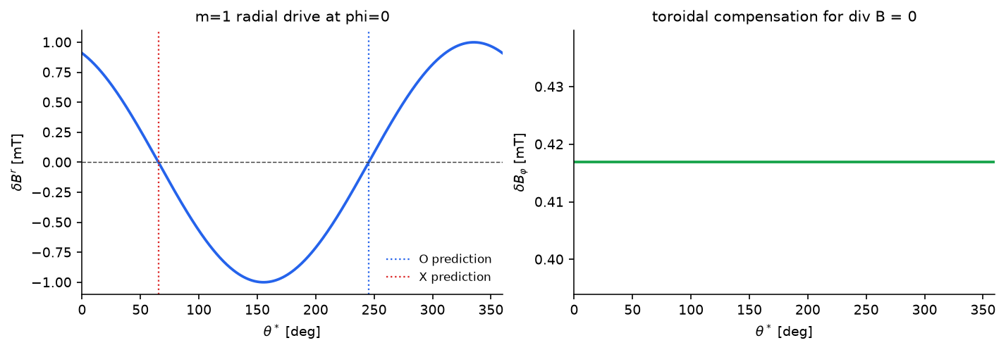
Die m=1-Störung tritt häufig genug auf, dass sie nicht als Randfall behandelt werden sollte. Hier treibt dasselbe divergenzfreie Template eine (1,1)-Resonanz in einem einfachen q=1-Gleichgewicht an. Wir prüfen in einer kurzen Berechnung drei Dinge: Das Feld ist numerisch solenoidal, die extrahierte Phase von b_{1,-1} folgt der Template-Phase, und die vorhergesagten O/X-Punkte liegen auf den Nulldurchgängen des radialen Antriebs.
[5]:
eq_m1 = simple_stellarator(
    R0=eq.R0,
    r0=eq.r0,
    B0=eq.B0,
    q0=0.75,
    q1=1.25,
    m_h=eq.m_h,
    n_h=eq.n_h,
    epsilon_h=0.0,
)
m1_phase = 0.43
delta_B_m1 = radial_rmp_field_template(
    1,
    1,
    amplitude=B_rmp,
    phase=m1_phase,
    axis_R=eq_m1.R0,
)
psi_res_m1 = eq_m1.resonant_psi(1, 1)[0]
r_res_m1 = np.sqrt(psi_res_m1) * eq_m1.r0
m1_diag = circular_shell_divergence_diagnostic(
    delta_B_m1,
    axis_R=eq_m1.R0,
    r_values=np.linspace(0.08, 0.28, 7),
    n_theta=192,
    n_phi=192,
)
component_m1 = find_resonant_components_analytic(
    eq_m1,
    delta_B_m1,
    base_m=1,
    base_n=1,
    max_harmonic=1,
    n_theta=128,
    n_phi=64,
    min_amplitude=1e-16,
)[0]

print(f'm=1 resonante Fläche: psi={psi_res_m1:.3f}, r={r_res_m1*100:.1f} cm')
print(f'arg b_(1,-1) = {np.angle(component_m1.b_mn):.6f} rad, Template-Phase = {m1_phase:.6f} rad')
print(f'|b_(1,-1)| = {abs(component_m1.b_mn):.3e} T, erwartet etwa B_rmp/2 = {0.5*B_rmp:.3e} T')
print(f'm=1 divergence relatives Maximum = {m1_diag.relative_max:.3e}')
print(f'O-Punkt theta = {np.degrees(component_m1.opoint_theta):.2f} deg')
print(f'X-Punkt theta = {np.degrees(component_m1.xpoint_theta):.2f} deg')

theta_m1 = np.linspace(0, 2*np.pi, 361)
R_m1 = eq_m1.R0 + r_res_m1*np.cos(theta_m1)
Z_m1 = r_res_m1*np.sin(theta_m1)
BR_m1, BZ_m1, Bphi_m1 = delta_B_m1(R_m1, Z_m1, 0.0)
dBr_m1 = BR_m1*np.cos(theta_m1) + BZ_m1*np.sin(theta_m1)

fig_m1, (ax_m1, ax_m1b) = plt.subplots(1, 2, figsize=(9.4, 3.2), constrained_layout=True)
ax_m1.plot(np.degrees(theta_m1), dBr_m1*1e3, color='#2563eb', lw=1.8)
ax_m1.axhline(0, color='0.25', lw=0.7, ls='--')
ax_m1.axvline(np.degrees(component_m1.opoint_theta), color='#2563eb', lw=1.1, ls=':', label='O-Vorhersage')
ax_m1.axvline(np.degrees(component_m1.xpoint_theta), color='#dc2626', lw=1.1, ls=':', label='X-Vorhersage')
ax_m1.set_xlim(0, 360)
ax_m1.set_xlabel(r'$\theta^*$ [deg]')
ax_m1.set_ylabel(r'$\delta B^r$ [mT]')
ax_m1.set_title('radialer m=1-Antrieb bei phi=0')
ax_m1.legend(frameon=False, fontsize=8)

ax_m1b.plot(np.degrees(theta_m1), Bphi_m1*1e3, color='#16a34a', lw=1.8)
ax_m1b.set_xlim(0, 360)
ax_m1b.set_xlabel(r'$\theta^*$ [deg]')
ax_m1b.set_ylabel(r'$\delta B_\varphi$ [mT]')
ax_m1b.set_title('toroidale Kompensation für div B = 0')
plt.show()
  k=1: (1,1) ψ_res=0.500 q_res=1.000 |b_mn|=5.000e-04 phase_arg=24.6° w_ψ=0.1265 (2.68 cm) θ_O=245.4° θ_X=65.4°
m=1 resonante Fläche: psi=0.500, r=21.2 cm
arg b_(1,-1) = 0.430000 rad, Template-Phase = 0.430000 rad
|b_(1,-1)| = 5.000e-04 T, erwartet etwa B_rmp/2 = 5.000e-04 T
m=1 divergence relatives Maximum = 9.946e-05
O-Punkt theta = 245.36 deg
X-Punkt theta = 65.36 deg
[RESONANT_COMPONENTS] Resonante Fourier-Komponenten finden#
Wir zerlegen das RMP-Feld auf jeder resonanten Flussfläche mit einer 2D-FFT und extrahieren die Amplituden der resonanten Harmonischen \((m_k, n_k) = k\times(2,1)\). Die Inselhalbbreite wird durch die Rutherford-Formel gegeben:
Ergebnisse werden in pyna_output/rmp_components.json zwischengespeichert.
[6]:
CACHE_COMP = pathlib.Path('pyna_output/rmp_components.json')
CACHE_COMP.parent.mkdir(exist_ok=True)

print('Berechne resonante Komponenten (n_theta=32, n_phi=16)...')
components = find_resonant_components_analytic(
    eq, delta_B_RMP, base_m=base_m, base_n=base_n,
    max_harmonic=3, n_theta=32, n_phi=16,
)
print(f'Gefunden: {len(components)} resonante Komponenten.')

# Cache as JSON
_comp_data = [{
    'm': c.m, 'n': c.n, 'harmonic_order': c.harmonic_order,
    'b_mn_real': float(c.b_mn.real), 'b_mn_imag': float(c.b_mn.imag),
    'psi_res': float(c.psi_res), 'q_res': float(c.q_res),
    'half_width_psi': float(c.half_width_psi),
    'half_width_r': float(c.half_width_r),
    'opoint_theta': float(c.opoint_theta),
    'xpoint_theta': float(c.xpoint_theta),
    'q_prime_sign': int(c.q_prime_sign),
} for c in components]
CACHE_COMP.write_text(json.dumps(_comp_data, indent=2))
print('Zwischengespeichert in', CACHE_COMP)

# Print table
print()
print(f'{"k":>3}  {"(m,n)":>8}  {"psi_res":>8}  {"q_res":>6}  {"b_mn|":>10}  {"w_psi":>8}  {"w_r (cm)":>10}  {"theta_O":>8}  {"theta_X":>8}')
print('-'*80)
for c in components:
    print(f'{c.harmonic_order:>3}  ({c.m},{c.n}){"":>4}  {c.psi_res:>8.4f}  {c.q_res:>6.3f}  {abs(c.b_mn):>10.3e}  {c.half_width_psi:>8.4f}  {c.half_width_r*100:>10.2f}  {np.degrees(c.opoint_theta):>8.1f}  {np.degrees(c.xpoint_theta):>8.1f}')
Berechne resonante Komponenten (n_theta=32, n_phi=16)...
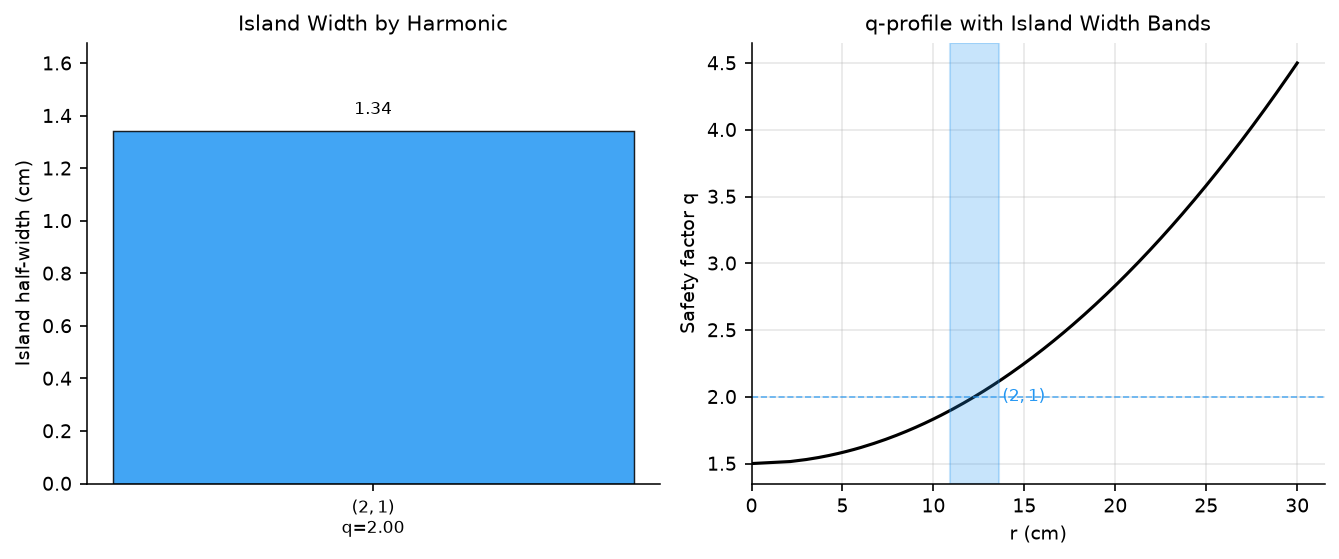
  k=1: (2,1) ψ_res=0.167 q_res=2.000 |b_mn|=5.000e-04 phase_arg=-0.0° w_ψ=0.0365 (1.34 cm) θ_O=135.0° θ_X=45.0°
  k=2: (4,2) — |b_mn|=4.57e-21 unter Schwellwert
  k=3: (6,3) — |b_mn|=1.98e-20 unter Schwellwert
Gefunden: 1 resonante Komponenten.
Zwischengespeichert in pyna_output/rmp_components.json

  k     (m,n)   psi_res   q_res       b_mn|     w_psi    w_r (cm)   theta_O   theta_X
--------------------------------------------------------------------------------
  1  (2,1)        0.1667   2.000   5.000e-04    0.0365        1.34     135.0      45.0
[POINCARE_PERTURBED] Geometrische Hochstufung: Kreuzungen -> X/O-Punkte -> Mannigfaltigkeiten#
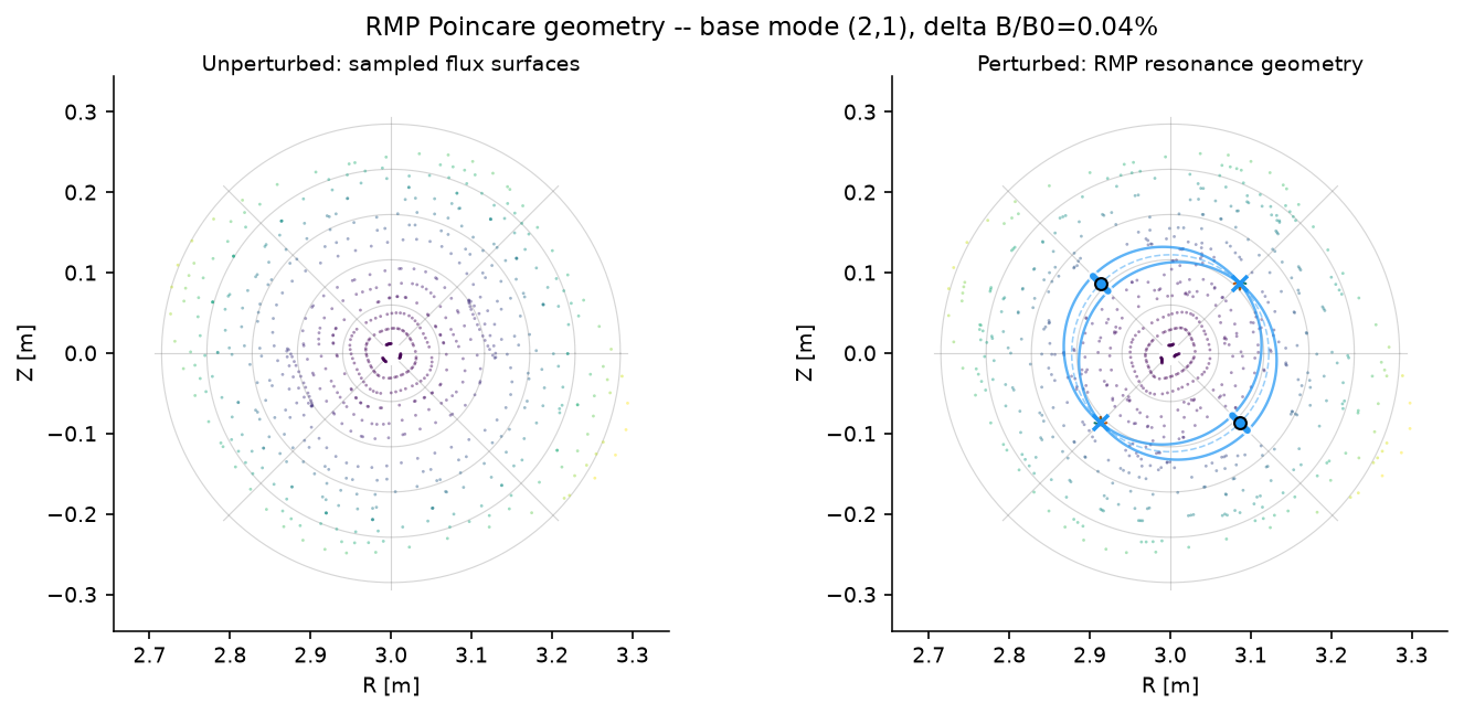
Die gestörte Verfolgung liefert abgetastete Poincaré-Punkte. Das analytische RMP-Spektrum liefert Fixpunkt- und Inselbreitenvorhersagen. pyna.plot.draw_rmp_resonance_section kombiniert sie zu einer Schnittgeometrie:
Poincaré-Punkte, eingefärbt nach Flusslabel;
PEST-artige \((S,\theta^*)\)-Gitterlinien;
resonante Flächen für jede Harmonische;
O-Punkte und X-Punkte aus der analytischen Fixpunktformel;
radiale O-Punkt-Balken, deren Länge durch die resonante Fourier-Amplitude bestimmt wird;
lokale stabile Separatrix-Äste, die aus den X-Punkten entstehen.
Dies ist dieselbe Hochstufungsidee wie im allgemeinen Geometrie-Workflow: Rohe Samples bleiben von persistenten geometrischen Objekten und Overlays getrennt, bis ein explizites Modell oder eine Diagnose die Hochstufung rechtfertigt.
[7]:
# Perturbed field_func
# --------------------
def field_func_perturbed(rzphi_1d):
    """Unit-tangent dRZphi/ds for the field-line ODE with RMP added."""
    rzphi_1d = np.asarray(rzphi_1d, dtype=float)
    R, Z, phi = rzphi_1d[0], rzphi_1d[1], rzphi_1d[2]
    theta = np.arctan2(Z, R - R0_eq)
    psi = eq.psi_ax(R, Z)
    q = float(eq.q_of_psi(psi))
    r_minor = np.sqrt((R - R0_eq)**2 + Z**2)
    B_phi = eq.B0 * eq.R0 / R
    B_pol = B_phi * r_minor / (R * max(abs(q), 1e-3))
    if r_minor > 1e-10:
        BR0 = -B_pol * np.sin(theta)
        BZ0 =  B_pol * np.cos(theta)
    else:
        BR0 = BZ0 = 0.0
    delta_BR_eq = eq.epsilon_h * eq.B0 * psi * np.cos(eq.m_h * theta - eq.n_h * phi)
    db = delta_B_RMP(R, Z, phi)
    BR_tot = BR0 + delta_BR_eq + db[0]
    BZ_tot = BZ0 + db[1]
    B_phi_tot = B_phi + db[2]
    B_mag = np.sqrt(BR_tot**2 + BZ_tot**2 + B_phi_tot**2) + 1e-30
    return np.array([BR_tot/B_mag, BZ_tot/B_mag, B_phi_tot/(R*B_mag)])

CACHE_PERT = pathlib.Path('pyna_output/poincare_perturbed_divfree.json')
CACHE_PERT.parent.mkdir(exist_ok=True)

phi_sections_deg = [0, 60, 120, 180, 240, 300]
phi_sections = np.array(phi_sections_deg) * np.pi / 180.0

if CACHE_PERT.exists():
    _d = json.loads(CACHE_PERT.read_text())
    all_sections_data = _d['sections']
    print(f'Gestörte Poincaré-Daten aus Cache geladen ({len(all_sections_data)} sections).')
else:
    sections_p = [ToroidalSection(phi0=ph) for ph in phi_sections]
    n_fieldlines, n_turns, dt = 15, 50, 0.08
    t_max = n_turns * 2 * np.pi * eq.R0
    start_pts = np.zeros((n_fieldlines, 3))
    start_pts[:, 0] = np.linspace(eq.R0 + 0.04*eq.r0, eq.R0 + 0.92*eq.r0, n_fieldlines)

    print(f'Verfolge {n_fieldlines} Feldlinien x {n_turns} Umläufe (t_max={t_max:.1f} m)...')
    pmap_p = poincare_from_fieldlines(field_func_perturbed, start_pts, sections_p, t_max=t_max, dt=dt)
    all_sections_data = []
    for i_sec, phi_deg in enumerate(phi_sections_deg):
        arr = pmap_p.crossing_array(i_sec)
        print(f'  phi={phi_deg} deg: {len(arr)} Kreuzungen')
        all_sections_data.append({'R': arr[:, 0].tolist() if len(arr) else [], 'Z': arr[:, 1].tolist() if len(arr) else []})
    CACHE_PERT.write_text(json.dumps({'phi_sections_deg': phi_sections_deg, 'sections': all_sections_data}))
    print('Berechnet und zwischengespeichert.')

R_cross_p0 = np.array(all_sections_data[0]['R'])
Z_cross_p0 = np.array(all_sections_data[0]['Z'])
print(f'phi=0 section: {len(R_cross_p0)} Kreuzungen')

fig2, (axL, axR) = plt.subplots(1, 2, figsize=(9.4, 4.2), constrained_layout=True)

# The low-level plot layers are independently selectable by name.
draw_rmp_resonance_section(
    axL,
    R_cross_u,
    Z_cross_u,
    eq=eq,
    components=[],
    phi=0.0,
    title='Ungestört: abgetastete Flussflächen',
    overlays=('pest_grid', 'poincare'),
    point_size=1.8,
    point_alpha=0.46,
)
draw_rmp_resonance_section(
    axR,
    R_cross_p0,
    Z_cross_p0,
    eq=eq,
    components=components,
    phi=0.0,
    colors=ISLAND_CMAPS,
    title='Gestört: RMP-Resonanzgeometrie',
    overlays=('pest_grid', 'poincare', 'resonant_Flächen', 'stable_branches', 'island_width_bars', 'xo'),
    point_size=1.8,
    point_alpha=0.46,
)

fig2.suptitle(
    f'RMP Poincaré geometry -- base Modus ({base_m},{base_n}), '
    f'delta B/B0={B_rmp/eq.B0*100:.2f}%',
    fontsize=11,
)
plt.show()
Gestörte Poincaré-Daten aus Cache geladen (6 sections).
phi=0 section: 735 Kreuzungen
[CYNA_FIXED_POINTS] Newton-Fixpunkte gegenüber RMP-Spektralphasen#
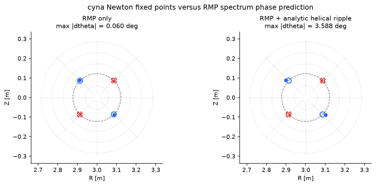
Das RMP-Spektrum sagt O/X-Punkt-Phasen erster Ordnung vorher. Hier verwenden wir die beschleunigte cyna-Newton-Karte, um diese Startwerte zu echten Fixpunkten periodischer Orbits zu verfeinern und dann den Phasenfehler zu messen. Der RMP-only-Fall ist ein Code-Sanity-Check; das Hinzufügen des analytischen helikalen Ripples zeigt die endliche Amplituden-/Modellverschiebung, die das Spektrum erster Ordnung absichtlich ignoriert.
[8]:
# Build a physical cylindrical field for cyna and compare Newton fixed points.
def row_newton_theta_deg(row, eq_case):
    axis_R, axis_Z = eq_case.magnetic_axis
    theta = np.arctan2(row.newton_Z - axis_Z, row.newton_R - axis_R) % (2*np.pi)
    return float(np.degrees(theta))


cyna_rows_by_case = {}
cyna_eq_by_case = {}
if components:
    eq_rmp_only = simple_stellarator(
        R0=eq.R0, r0=eq.r0, B0=eq.B0,
        q0=eq.q0, q1=eq.q1,
        m_h=eq.m_h, n_h=eq.n_h, epsilon_h=0.0,
    )
    try:
        for case_label, eq_case in [
            ('nur RMP', eq_rmp_only),
            ('RMP + analytisches helikales Ripple', eq),
        ]:
            print(f'Baue cyna-Feld: {case_label}')
            field_case = sample_stellarator_cylindrical_field(
                eq_case,
                delta_B_RMP,
                nR=128,
                nPhi=128,
                label=f'analytic_rmp_for_cyna_{case_label.replace(" ", "_").lower()}',
            )
            rows = compare_cyna_fixed_points_for_component(
                field_case,
                components[0],
                eq_case,
                DPhi=0.015,
                max_iter=80,
                tol=1e-11,
                n_threads=4,
            )
            cyna_rows_by_case[case_label] = rows
            cyna_eq_by_case[case_label] = eq_case
    except ImportError as exc:
        print('cyna-Fixpunktvergleich übersprungen:', exc)

if cyna_rows_by_case:
    print()
    header = '{:<30} {:>4} {:>6} {:>9} {:>9} {:>10} {:>11} {:>11} {:>11}'.format(
        'case', 'kind', 'branch', 'theta*', 'theta_N', 'dtheta', 'm*dtheta', 'dr [cm]', 'residual'
    )
    print(header)
    print('-' * len(header))
    for case_label, rows in cyna_rows_by_case.items():
        eq_case = cyna_eq_by_case[case_label]
        for row in rows:
            theta_n = row_newton_theta_deg(row, eq_case)
            print('{:<30} {:>4} {:>6d} {:>9.3f} {:>9.3f} {:>10.4f} {:>11.4f} {:>11.4f} {:>11.1e}'.format(
                case_label,
                row.predicted_kind + '/' + (row.newton_kind or '?'),
                row.branch,
                row.predicted_theta_deg,
                theta_n,
                row.theta_error_deg,
                row.helical_phase_error_deg,
                row.radial_error_cm,
                row.residual,
            ))
        max_dtheta = max(abs(row.theta_error_deg) for row in rows)
        max_helical = max(abs(row.helical_phase_error_deg) for row in rows)
        print(f'  -> {case_label}: max |dtheta|={max_dtheta:.4f} deg, max |m*dtheta|={max_helical:.4f} deg')

if cyna_rows_by_case:
    fig_cmp, axes_cmp = plt.subplots(1, len(cyna_rows_by_case), figsize=(9.2, 4.0), constrained_layout=True)
    axes_cmp = np.atleast_1d(axes_cmp)
    for ax, (case_label, rows) in zip(axes_cmp, cyna_rows_by_case.items()):
        eq_case = cyna_eq_by_case[case_label]
        draw_pest_grid(ax, eq_case, alpha=0.18)
        r_res = np.sqrt(components[0].psi_res) * eq_case.r0
        theta_ring = np.linspace(0, 2*np.pi, 361)
        ax.plot(eq_case.R0 + r_res*np.cos(theta_ring), r_res*np.sin(theta_ring),
                color='0.25', lw=0.9, ls='--', alpha=0.65)
        for row in rows:
            color = '#2563eb' if row.predicted_kind == 'O' else '#dc2626'
            marker = 'o' if row.predicted_kind == 'O' else 'X'
            ax.plot([row.predicted_R, row.newton_R], [row.predicted_Z, row.newton_Z],
                    color=color, lw=1.0, alpha=0.65)
            ax.scatter(row.predicted_R, row.predicted_Z, marker=marker, s=70,
                       facecolors='none', edgecolors=color, linewidths=1.3, zorder=5)
            ax.scatter(row.newton_R, row.newton_Z, marker=marker, s=42,
                       color=color, edgecolors='white', linewidths=0.5, zorder=6)
        lim = 1.12 * eq_case.r0
        ax.set_xlim(eq_case.R0 - lim, eq_case.R0 + lim)
        ax.set_ylim(-lim, lim)
        ax.set_aspect('equal')
        ax.set_xlabel('R [m]')
        ax.set_ylabel('Z [m]')
        max_dtheta = max(abs(row.theta_error_deg) for row in rows)
        ax.set_title(f'{case_label}\nmax |dtheta| = {max_dtheta:.3f} deg')
    fig_cmp.suptitle('cyna-Newton-Fixpunkte gegenüber RMP-Spektralphasenvorhersage', fontsize=11)
    plt.show()
Baue cyna-Feld: nur RMP
Baue cyna-Feld: RMP + analytisches helikales Ripple

case                           kind branch    theta*   theta_N     dtheta    m*dtheta     dr [cm]    residual
-------------------------------------------------------------------------------------------------------------
nur RMP                        O/O      0   315.000   314.940    -0.0602     -0.1203      0.2298     1.4e-14
nur RMP                        O/O      1   135.000   135.059     0.0588      0.1176      0.2303     9.2e-15
nur RMP                        X/X      0    45.000    44.940    -0.0600     -0.1200     -0.2520     4.7e-14
nur RMP                        X/X      1   225.000   225.059     0.0588      0.1176     -0.2515     1.7e-14
  -> nur RMP: max |dtheta|=0.0602 deg, max |m*dtheta|=0.1203 deg
RMP + analytisches helikales Ripple   O/O      0   315.000   318.588     3.5877      7.1754      1.2050     5.0e-12
RMP + analytisches helikales Ripple   O/O      1   135.000   138.420     3.4195      6.8391      1.1869     2.2e-15
RMP + analytisches helikales Ripple   X/X      0    45.000    47.043     2.0428      4.0857     -0.2143     2.7e-12
RMP + analytisches helikales Ripple   X/X      1   225.000   226.940     1.9400      3.8801     -0.2445     2.3e-12
  -> RMP + analytisches helikales Ripple: max |dtheta|=3.5877 deg, max |m*dtheta|=7.1754 deg
[NONRESONANT_DEFORMATION] Nichtresonantes Ripple als Flussflächenverformung#
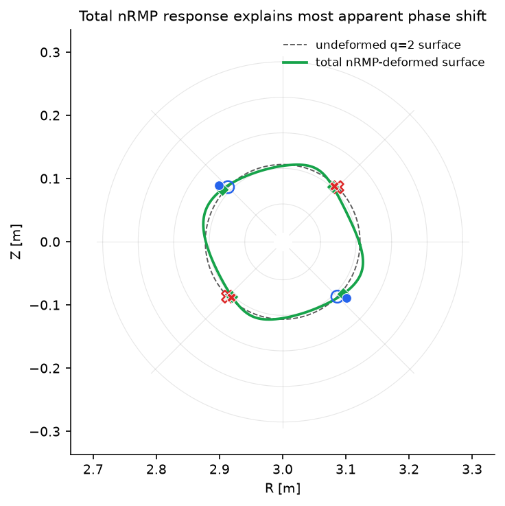
Das helikale Ripple in diesem analytischen Gleichgewicht ist nicht die resonante RMP-Komponente, die die (m,n)=(2,1)-Insel öffnet. Es verändert dennoch die Geometrie der benachbarten Flussfläche. Wenn Newton-Fixpunkte mit der unverformten Kreisfläche verglichen werden, erscheint diese glatte Verschiebung als künstlicher Phasenfehler.
Wir tasten hier den Beitrag des helikalen Ripples zur Feldlinien-ODE ab,
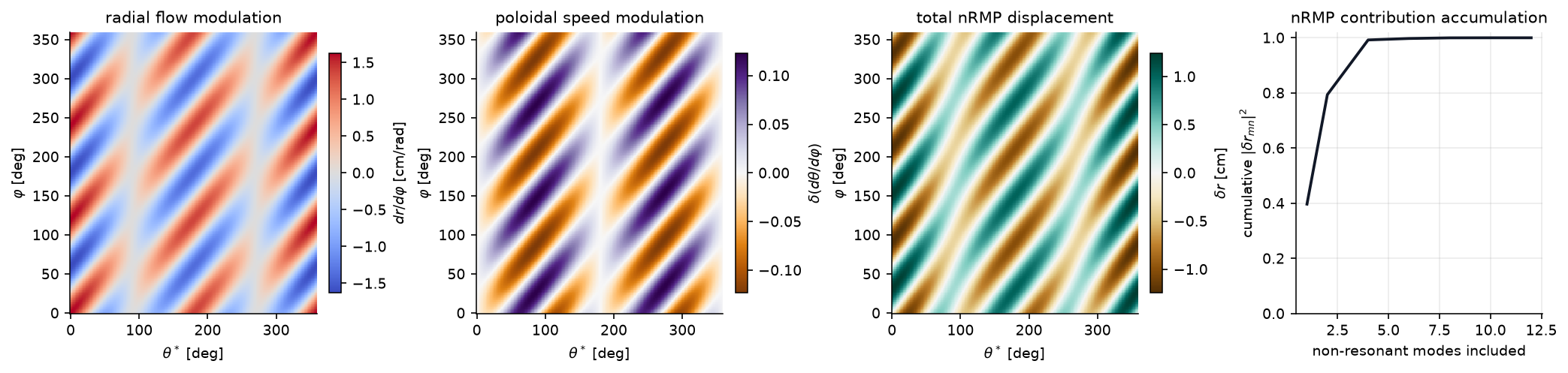
Fourier-transformieren F_r und F_theta und lösen für jeden nichtresonanten Koeffizienten die nichtresonante homologische Gleichung. Das Antwortobjekt enthält die Gesamtverformung und eine Beitragsrangliste; die Rangliste ist eine Diagnose, während die unten verwendete Verformung die vollständig aufsummierte nRMP-Antwort ist.
[9]:
def helical_ripple_delta_B(eq_case):
    """Return the analytic helical-ripple contribution used by simple_stellarator."""
    def delta_B_helical(R, Z, phi):
        R_arr = np.asarray(R, dtype=float)
        Z_arr = np.asarray(Z, dtype=float)
        phi_arr = np.asarray(phi, dtype=float)
        theta = np.arctan2(Z_arr, R_arr - eq_case.R0)
        psi = eq_case.psi_ax(R_arr, Z_arr)
        dBR = eq_case.epsilon_h * eq_case.B0 * psi * np.cos(eq_case.m_h * theta - eq_case.n_h * phi_arr)
        return np.array([
            dBR,
            np.zeros_like(dBR, dtype=float),
            np.zeros_like(dBR, dtype=float),
        ])
    return delta_B_helical


def helical_velocity_response(eq_case, psi_res, n_theta=256, n_phi=256, include_shear=False):
    velocity = fieldline_velocity_spectrum_on_circular_surface(
        eq_case,
        helical_ripple_delta_B(eq_case),
        psi_res,
        n_theta=n_theta,
        n_phi=n_phi,
        m_max=8,
        n_max=8,
        min_amplitude=1e-12,
    )
    return velocity.nonresonant_response(include_shear=include_shear)


def helical_velocity_deformation(eq_case, psi_res, n_theta=256, n_phi=256, include_shear=False):
    response = helical_velocity_response(
        eq_case,
        psi_res,
        n_theta=n_theta,
        n_phi=n_phi,
        include_shear=include_shear,
    )
    return response.deformation, response.velocity.r_minor, response.velocity


case_label = 'RMP + analytisches helikales Ripple'
if components and case_label in cyna_rows_by_case:
    rows = cyna_rows_by_case[case_label]
    eq_case = cyna_eq_by_case[case_label]
    response_helical = helical_velocity_response(eq_case, components[0].psi_res)
    deformation = response_helical.deformation
    velocity_helical = response_helical.velocity
    r_res = velocity_helical.r_minor
    projected_rows = project_fixed_points_to_deformed_surface(
        rows,
        eq_case,
        deformation,
        r_minor=r_res,
        theta_window=0.35,
    )

    print(
        'nRMP-Gesamtantwort verwendet '
        f'{response_helical.n_nonresonant_Moduss} non-resonant Moduss '
        f'and excludes {response_helical.n_resonant_Moduss} resonante Moden aus.'
    )
    print('Größte nRMP-Antwortbeiträge; sie ordnen die Summe, ersetzen sie aber nicht:')
    print('{:>8} {:>12} {:>14} {:>14}'.format('(m,n)', 'detuning', '|delta_r_mn| cm', 'cum frac'))
    for contrib in response_helical.contribution_rows(top=6):
        print('({:>2d},{:>2d}) {:>12.3e} {:>14.4f} {:>14.3f}'.format(
            contrib.m,
            contrib.n,
            contrib.detuning,
            100.0 * contrib.radial_response_weight,
            contrib.cumulative_fraction,
        ))
    print()

    raw_max = max(abs(row.theta_error_deg) for row in rows)
    corrected_max = max(abs(row.theta_error_deg) for row in projected_rows)
    nearest_max = max(row.distance_cm for row in projected_rows)
    print(f'Rohwert Kreisfläche max |dtheta|:       {raw_max:.4f} deg')
    print(f'Verformte-Flächen-Koordinate max |dtheta|: {corrected_max:.4f} deg')
    print(f'Max. Abstand Newton zu verformtem Schnitt:  {nearest_max:.3f} cm')
    print()
    header = '{:<4} {:>6} {:>12} {:>16} {:>13}'.format(
        'kind', 'branch', 'raw dtheta', 'deformed dtheta', 'distance [cm]'
    )
    print(header)
    print('-' * len(header))
    for row, proj in zip(rows, projected_rows):
        print('{:<4} {:>6d} {:>12.4f} {:>16.4f} {:>13.3f}'.format(
            row.predicted_kind,
            row.branch,
            row.theta_error_deg,
            proj.theta_error_deg,
            proj.distance_cm,
        ))

    theta_line = np.linspace(0.0, 2*np.pi, 721)
    R_circ = eq_case.R0 + r_res*np.cos(theta_line)
    Z_circ = r_res*np.sin(theta_line)
    R_def, Z_def = deformed_circular_section_rz(eq_case, r_res, deformation, theta_line)

    fig_def, ax_def = plt.subplots(figsize=(5.2, 4.8), constrained_layout=True)
    draw_pest_grid(ax_def, eq_case, alpha=0.16)
    ax_def.plot(R_circ, Z_circ, color='0.35', lw=0.9, ls='--', label='unverformte q=2-Fläche')
    ax_def.plot(R_def, Z_def, color='#16a34a', lw=1.8, label='gesamte nRMP-verformte Fläche')

    for row, proj in zip(rows, projected_rows):
        color = '#2563eb' if row.predicted_kind == 'O' else '#dc2626'
        marker = 'o' if row.predicted_kind == 'O' else 'X'
        ax_def.plot([row.predicted_R, row.newton_R], [row.predicted_Z, row.newton_Z],
                    color=color, lw=0.8, alpha=0.35)
        ax_def.plot([proj.closest_R, row.newton_R], [proj.closest_Z, row.newton_Z],
                    color=color, lw=1.1, ls=':', alpha=0.9)
        ax_def.scatter(row.predicted_R, row.predicted_Z, marker=marker, s=72,
                       facecolors='none', edgecolors=color, linewidths=1.2, zorder=5)
        ax_def.scatter(proj.closest_R, proj.closest_Z, marker='D', s=42,
                       color='#16a34a', edgecolors='white', linewidths=0.45, zorder=6)
        ax_def.scatter(row.newton_R, row.newton_Z, marker=marker, s=44,
                       color=color, edgecolors='white', linewidths=0.5, zorder=7)

    lim = 1.12 * eq_case.r0
    ax_def.set_xlim(eq_case.R0 - lim, eq_case.R0 + lim)
    ax_def.set_ylim(-lim, lim)
    ax_def.set_aspect('equal')
    ax_def.set_xlabel('R [m]')
    ax_def.set_ylabel('Z [m]')
    ax_def.set_title('Gesamte nRMP-Antwort erklärt den größten Teil der scheinbaren Phasenverschiebung')
    ax_def.legend(frameon=False, loc='upper right', fontsize=8)
    plt.show()

    TT_h, PP_h, dr_h, dtheta_h = response_helical.real_fields()
    counts_h, cumulative_h = response_helical.cumulative_contribution()
    theta_deg_h = np.degrees(velocity_helical.theta)
    phi_deg_h = np.degrees(velocity_helical.phi)
    fig_flow, axes_flow = plt.subplots(1, 4, figsize=(13.8, 3.2), constrained_layout=True)
    panels = [
        (velocity_helical.radial_velocity * 100.0, r'$dr/d\varphi$ [cm/rad]', 'radial flow modulation', 'coolwarm'),
        (velocity_helical.poloidal_velocity, r'$\delta(d\theta/d\varphi)$', 'poloidal speed modulation', 'PuOr'),
        (dr_h * 100.0, r'$\delta r$ [cm]', 'total nRMP displacement', 'BrBG'),
    ]
    for ax, (data, cbar_label, title, cmap) in zip(axes_flow[:3], panels):
        vmax = np.nanmax(np.abs(data))
        im = ax.pcolormesh(
            theta_deg_h,
            phi_deg_h,
            data,
            shading='auto',
            cmap=cmap,
            vmin=-vmax,
            vmax=vmax,
        )
        ax.set_xlabel(r'$\theta^*$ [deg]')
        ax.set_ylabel(r'$\varphi$ [deg]')
        ax.set_title(title)
        fig_flow.colorbar(im, ax=ax, label=cbar_label, shrink=0.85)
    axes_flow[3].plot(counts_h, cumulative_h, color='#111827', lw=1.8)
    axes_flow[3].set_ylim(0, 1.02)
    axes_flow[3].set_xlabel('einbezogene nichtresonante Moden')
    axes_flow[3].set_ylabel(r'cumulative $|\delta r_{mn}|^2$')
    axes_flow[3].set_title('Akkumulation der nRMP-Beiträge')
    axes_flow[3].grid(True, alpha=0.25)
    plt.show()
else:
    print('Non-resonant deformation check skipped because cyna rows are unavailable.')
nRMP-Gesamtantwort verwendet 12 nichtresonante Moden und schließt 2 resonante Moden aus.
Größte nRMP-Antwortbeiträge; sie ordnen die Summe, ersetzen sie aber nicht:
   (m,n)     detuning |delta_r_mn| cm       cum frac
(-4, 3)    1.000e+00         0.3755          0.397
( 4,-3)   -1.000e+00         0.3755          0.794
(-2, 3)    2.000e+00         0.1877          0.893
( 2,-3)   -2.000e+00         0.1877          0.992
(-5, 3)    5.000e-01         0.0306          0.995
( 5,-3)   -5.000e-01         0.0306          0.997

Rohwert Kreisfläche max |dtheta|:       3.5877 deg
Verformte-Flächen-Koordinate max |dtheta|: 1.4748 deg
Max. Abstand Newton zu verformtem Schnitt:  0.822 cm

kind branch   raw dtheta  deformed dtheta distance [cm]
-------------------------------------------------------
O         0       3.5877           0.6159         0.822
O         1       3.4195           0.7933         0.783
X         0       2.0428          -1.4748         0.250
X         1       1.9400          -1.1567         0.196
[MIXED_SPECTRUM] Gemischter RMP/nRMP-Workflow auf einer Fläche#
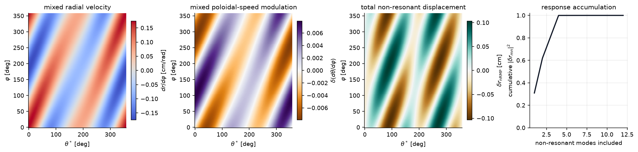
Reale Störungen enthalten selten nur eine saubere Harmonische. Dieses Beispiel überlagert eine resonante (2,1)-RMP mit zwei nichtresonanten Komponenten, darunter ein m=1-Term. Die Modentabelle klassifiziert das abgetastete Geschwindigkeitsspektrum, ist aber nur eine Diagnose. Der nRMP-Teil der Berechnung ist das gesamte Antwortobjekt, das jede nichtresonante Zeile summiert, bevor glatte Verschiebung und Geschwindigkeitsmodulation gezeichnet werden.
[10]:
mixed_delta_B = compose_magnetic_perturbations(
    delta_B_RMP,
    radial_rmp_field_template(3, 1, amplitude=2.0e-4, phase=0.20, axis_R=eq.R0),
    radial_rmp_field_template(1, 1, amplitude=1.5e-4, phase=0.40, axis_R=eq.R0),
)

mixed_velocity = fieldline_velocity_spectrum_on_circular_surface(
    eq,
    mixed_delta_B,
    psi_res_21,
    n_theta=160,
    n_phi=128,
    m_max=5,
    n_max=4,
    min_amplitude=1e-13,
)
mixed_rows = rmp_nrmp_Modus_rows(
    mixed_velocity.radial_spectrum,
    mixed_velocity.iota,
    resonance_tol=1e-10,
    top=12,
    min_amplitude=1e-8,
)
mixed_response = mixed_velocity.nonresonant_response(include_shear=True, resonance_tol=1e-10)

print(f'Lokales iota auf q=2-Fläche: {mixed_velocity.iota:.6f}')
print(
    'Gesamte nRMP-Antwort verwendet '
    f'{mixed_response.n_nonresonant_Moduss} non-resonant Moduss; '
    f'{mixed_response.n_resonant_Moduss} resonante Moden bleiben für die Inselanalyse.'
)
print()
print('RMP/nRMP-Modenklassifikationsdiagnose:')
print('{:<5} {:>8} {:>12} {:>12} {:>12}'.format('kind', '(m,n)', 'detuning', '|F_r mn|', 'phase [deg]'))
print('-' * 56)
for row in mixed_rows:
    print('{:<5} ({:>2d},{:>2d}) {:>12.3e} {:>12.3e} {:>12.2f}'.format(
        row.kind,
        row.m,
        row.n,
        row.detuning,
        row.amplitude,
        row.phase_deg,
    ))

print()
print('Größte Beiträge zur gesamten radialen nRMP-Antwort:')
print('{:>8} {:>12} {:>14} {:>14}'.format('(m,n)', 'detuning', '|delta_r_mn| cm', 'cum frac'))
for contrib in mixed_response.contribution_rows(top=8):
    print('({:>2d},{:>2d}) {:>12.3e} {:>14.4f} {:>14.3f}'.format(
        contrib.m,
        contrib.n,
        contrib.detuning,
        100.0 * contrib.radial_response_weight,
        contrib.cumulative_fraction,
    ))

mixed_deformation = mixed_response.deformation
TT_mix, PP_mix, nonres_dr_mix, nonres_dtheta_mix = mixed_response.real_fields()
counts_mix, cumulative_mix = mixed_response.cumulative_contribution()

theta_deg_mix = np.degrees(mixed_velocity.theta)
phi_deg_mix = np.degrees(mixed_velocity.phi)
fig_mix, axes_mix = plt.subplots(1, 4, figsize=(13.8, 3.2), constrained_layout=True)
panels = [
    (mixed_velocity.radial_velocity * 100.0, r'$dr/d\varphi$ [cm/rad]', 'mixed radial velocity', 'coolwarm'),
    (mixed_velocity.poloidal_velocity, r'$\delta(d\theta/d\varphi)$', 'mixed poloidal-speed modulation', 'PuOr'),
    (nonres_dr_mix * 100.0, r'$\delta r_\mathrm{nRMP}$ [cm]', 'total non-resonant displacement', 'BrBG'),
]
for ax, (data, label, title, cmap) in zip(axes_mix[:3], panels):
    vmax = np.nanmax(np.abs(data))
    im = ax.pcolormesh(
        theta_deg_mix,
        phi_deg_mix,
        data,
        shading='auto',
        cmap=cmap,
        vmin=-vmax,
        vmax=vmax,
    )
    ax.set_xlabel(r'$\theta^*$ [deg]')
    ax.set_ylabel(r'$\varphi$ [deg]')
    ax.set_title(title)
    fig_mix.colorbar(im, ax=ax, label=label, shrink=0.86)
axes_mix[3].plot(counts_mix, cumulative_mix, color='#111827', lw=1.8)
axes_mix[3].set_ylim(0, 1.02)
axes_mix[3].set_xlabel('einbezogene nichtresonante Moden')
axes_mix[3].set_ylabel(r'cumulative $|\delta r_{mn}|^2$')
axes_mix[3].set_title('Antwortakkumulation')
axes_mix[3].grid(True, alpha=0.25)
plt.show()
Lokales iota auf q=2-Fläche: 0.500000
Gesamte nRMP-Antwort verwendet 12 non-resonant Moduss; 2 resonante Moden bleiben für die Inselanalyse.

RMP/nRMP-Modenklassifikationsdiagnose:
kind     (m,n)     detuning     |F_r mn|  phase [deg]
--------------------------------------------------------
RMP   (-2, 1)    0.000e+00    6.087e-04        -0.23
RMP   ( 2,-1)    0.000e+00    6.087e-04         0.23
nRMP  (-3, 1)   -5.000e-01    1.442e-04        -9.53
nRMP  ( 3,-1)    5.000e-01    1.442e-04         9.53
nRMP  (-1, 1)    5.000e-01    1.131e-04       -18.07
nRMP  ( 1,-1)   -5.000e-01    1.131e-04        18.07
nRMP  ( 4,-1)    1.000e+00    5.144e-06        10.91
nRMP  (-4, 1)   -1.000e+00    5.144e-06       -10.91
nRMP  ( 0,-1)   -1.000e+00    3.906e-06        21.49
nRMP  ( 0, 1)    1.000e+00    3.906e-06       -21.49
nRMP  (-5, 1)   -1.500e+00    5.000e-08       -11.46
nRMP  ( 5,-1)    1.500e+00    5.000e-08        11.46

Größte Beiträge zur gesamten radialen nRMP-Antwort:
   (m,n)     detuning |delta_r_mn| cm       cum frac
(-3, 1)   -5.000e-01         0.0288          0.310
( 3,-1)    5.000e-01         0.0288          0.619
(-1, 1)    5.000e-01         0.0226          0.809
( 1,-1)   -5.000e-01         0.0226          1.000
( 4,-1)    1.000e+00         0.0005          1.000
(-4, 1)   -1.000e+00         0.0005          1.000
( 0, 1)    1.000e+00         0.0004          1.000
( 0,-1)   -1.000e+00         0.0004          1.000
[ORDER_ANALYSIS] Prüfungen der Störungsordnung#
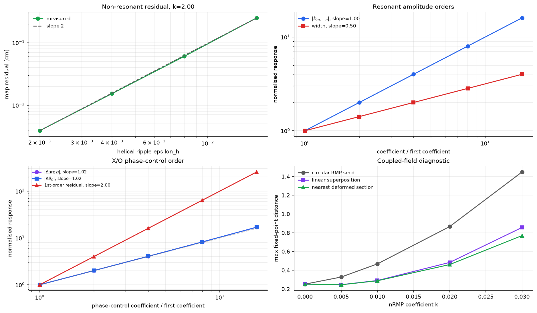
Der wiederverwendbare Workflow lebt jetzt in einigen kleinen Helpern: scan_nonresonant_residual_order, scan_rmp_amplitude_order, scan_rmp_phase_order, scan_rmp_resolution_convergence und plot_perturbation_order_summary.
Sobald die Fourier-Konvention festliegt, sind die erwarteten Ordnungen einfach:
nRMP-Flächenform-Residuum: Eine Verformung erster Ordnung sollte ein
O(k^2)-Kartenresiduum hinterlassen.RMP-resonanter Koeffizient: Für
delta B = k fliefert Fourier-Linearität|b_{m,-n}| ~ k.Inselbreite: Die Rutherford/Nardon-Pendelbreite skaliert wie
w ~ sqrt(|b_{m,-n}|), alsow ~ k^{1/2}.X/O-Phase: Die Phase wird von
arg(b_{m,-n})gesteuert, nicht von der Amplitude. Die exakte Beziehung lautetm*Delta theta_O + Delta arg(b_{m,-n}) = 0.
Für die Ordnung der Phasensteuerung verwenden wir das divergenzfreie Template radial_rmp_field_template. Sein Phasenparameter verändert die Phase des resonanten Koeffizienten, während div(delta B)=0 erhalten bleibt, einschließlich des wichtigen m=1-Falls. Wir testen absichtlich eine leicht nichtlineare Steuerphase alpha(k)=k+eta*k^2; das Residuum gegenüber dem Roh-k-Gesetz erster Ordnung sollte daher wie O(k^2) skalieren.
[11]:
def component_for_rmp_template(amplitude=1.0e-3, phase=0.0, n_theta=128, n_phi=64):
    return find_resonant_components_analytic(
        eq,
        radial_rmp_field_template(base_m, base_n, amplitude=amplitude, phase=phase, axis_R=eq.R0),
        base_m=base_m,
        base_n=base_n,
        max_harmonic=1,
        n_theta=n_theta,
        n_phi=n_phi,
        min_amplitude=1e-16,
        verbose=False,
    )[0]


def deformed_torus_map_residual(epsilon_h, n_alpha=12):
    eq_case = simple_stellarator(
        R0=eq.R0, r0=eq.r0, B0=eq.B0,
        q0=eq.q0, q1=eq.q1,
        m_h=eq.m_h, n_h=eq.n_h, epsilon_h=float(epsilon_h),
    )
    psi_res = eq_case.resonant_psi(base_m, base_n)[0]
    deformation, r_res, _ = helical_velocity_deformation(
        eq_case, psi_res, n_theta=128, n_phi=128, include_shear=True
    )
    iota = 1.0 / float(eq_case.q_of_psi(psi_res))

    def surface(alpha, phi):
        alpha_arr = np.asarray(alpha)
        return (
            r_res + deformation.section_r(alpha_arr, phi),
            alpha_arr + deformation.section_theta(alpha_arr, phi),
        )

    def rhs(phi, state):
        radius, theta = state
        R = eq_case.R0 + radius*np.cos(theta)
        psi_here = (radius / eq_case.r0)**2
        q_here = float(eq_case.q_of_psi(psi_here))
        Bphi = eq_case.B0 * eq_case.R0 / R
        delta_BR = eq_case.epsilon_h * eq_case.B0 * psi_here * np.cos(eq_case.m_h * theta - eq_case.n_h * phi)
        return [
            R * delta_BR * np.cos(theta) / Bphi,
            1.0/q_here - R * delta_BR * np.sin(theta) / (radius * Bphi),
        ]

    residual = deformed_surface_map_residual(
        surface,
        rhs,
        iota,
        alpha_values=np.linspace(0.0, 2*np.pi, n_alpha, endpoint=False),
        state_to_cartesian=lambda state, phi: [
            eq_case.R0 + float(state[0])*np.cos(float(state[1])),
            float(state[0])*np.sin(float(state[1])),
        ],
    )
    return residual.max_residual


def max_helical_deformation_cm(n_theta, n_phi):
    velocity = fieldline_velocity_spectrum_on_circular_surface(
        eq,
        helical_ripple_delta_B(eq),
        psi_res_21,
        n_theta=max(64, n_theta),
        n_phi=max(64, n_phi),
        m_max=8,
        n_max=8,
        min_amplitude=1e-12,
    )
    deformation = velocity.nonresonant_deformation(include_shear=True)
    TT, PP = np.meshgrid(velocity.theta, velocity.phi, indexing='xy')
    return 100.0 * float(np.nanmax(np.abs(deformation.real_field_r(TT, PP))))


nonres_eps = np.array([0.002, 0.004, 0.008, 0.016])
rmp_k = np.array([2.5e-4, 5e-4, 1e-3, 2e-3, 4e-3])
phase_controls = np.array([0.01, 0.02, 0.04, 0.08, 0.16])
phase_eta = 0.4

nonres_scan = scan_nonresonant_residual_order(nonres_eps, deformed_torus_map_residual)
rmp_amp_scan = scan_rmp_amplitude_order(
    rmp_k,
    lambda k: component_for_rmp_template(amplitude=k, phase=0.0, n_theta=64, n_phi=32),
)
phase_base = component_for_rmp_template(amplitude=1e-3, phase=0.0, n_theta=128, n_phi=64)
phase_scan = scan_rmp_phase_order(
    phase_controls,
    lambda k: component_for_rmp_template(
        amplitude=1e-3,
        phase=float(k) + phase_eta*float(k)*float(k),
        n_theta=128,
        n_phi=64,
    ),
    base_component=phase_base,
)
resolution_scan = scan_rmp_resolution_convergence(
    [(32, 16), (64, 32), (128, 64), (256, 128)],
    lambda n_theta, n_phi: component_for_rmp_template(
        amplitude=1e-3, phase=0.0, n_theta=n_theta, n_phi=n_phi
    ),
    deformation_metric_factory=max_helical_deformation_cm,
)

comp_pos = component_for_rmp_template(amplitude=1e-3, phase=0.0, n_theta=64, n_phi=32)
comp_neg = component_for_rmp_template(amplitude=-1e-3, phase=0.0, n_theta=64, n_phi=32)
sign_phase_jump_deg = float(np.degrees(np.angle(comp_neg.b_mn / comp_pos.b_mn)))

print(f'Steigung des nichtresonanten Verformungsresiduums = {nonres_scan.slope:.3f} (erwartet 2)')
print(f'Positive RMP: |b_mn| slope =             {rmp_amp_scan.b_fit.slope:.3f} (erwartet 1)')
print(f'Positive RMP: Steigung der Inselhalbbreite =  {rmp_amp_scan.width_fit.slope:.3f} (erwartet 0.5)')
print(f'Positive RMP: X/O-Phasenspanne:           {rmp_amp_scan.phase_span_deg:.3e} deg')
print(f'Negativer Koeffizient: Argsprung:         {sign_phase_jump_deg:.1f} deg')
print(f'  +k: O={np.degrees(comp_pos.opoint_theta):.1f} deg, X={np.degrees(comp_pos.xpoint_theta):.1f} deg')
print(f'  -k: O={np.degrees(comp_neg.opoint_theta):.1f} deg, X={np.degrees(comp_neg.xpoint_theta):.1f} deg')
print(f'Phasentemplate: |Delta arg b| slope =    {phase_scan.b_phase_fit.slope:.3f} (lokal erwartet 1)')
print(f'Phasentemplate: |Delta theta_O| vs |Delta arg b| slope = {phase_scan.opoint_vs_b_phase_fit.slope:.3f} (erwartet 1)')
print(f'Phasentemplate: max |m Delta theta_O + Delta arg b|: {phase_scan.max_exact_relation_residual:.3e} rad')
print(f'Phasentemplate: first-order residual slope = {phase_scan.first_order_residual_fit.slope:.3f} (erwartet 2)')

print()
print('Auflösungskonvergenz gegen das feinste RMP-Spektrumgitter:')
print('{:>8} {:>6} {:>12} {:>14} {:>14} {:>14}'.format(
    'n_theta', 'n_phi', 'rel |b| err', 'phase err deg', 'rel width err', 'max |dr| cm'
))
for row in resolution_scan.rows:
    print(f'{row.n_theta:8d} {row.n_phi:6d} {row.relative_b_error:12.3e} '
          f'{row.phase_error_deg:14.3e} {row.relative_width_error:14.3e} '
          f'{row.deformation_metric:14.4f}')

coupling_sweep = None
if components:
    component = components[0]

    def coupled_distances(eps_h):
        eq_case = simple_stellarator(
            R0=eq.R0, r0=eq.r0, B0=eq.B0,
            q0=eq.q0, q1=eq.q1,
            m_h=eq.m_h, n_h=eq.n_h, epsilon_h=float(eps_h),
        )
        rows = compare_cyna_fixed_points_for_component(
            sample_stellarator_cylindrical_field(
                eq_case, delta_B_RMP, nR=128, nPhi=128, label=f'coupled_rmp_eps_{eps_h:.3f}',
            ),
            component,
            eq_case,
            DPhi=0.015,
            max_iter=80,
            tol=1e-11,
            n_threads=4,
        )
        raw_cm = max(np.hypot(row.newton_R - row.predicted_R, row.newton_Z - row.predicted_Z) for row in rows) * 100.0
        if eps_h == 0.0:
            return raw_cm, raw_cm, raw_cm
        deformation, r_res, _ = helical_velocity_deformation(eq_case, component.psi_res, include_shear=True)
        superposed_cm = max(
            np.hypot(
                float(deformed_circular_section_rz(eq_case, r_res, deformation, row.predicted_theta)[0]) - row.newton_R,
                float(deformed_circular_section_rz(eq_case, r_res, deformation, row.predicted_theta)[1]) - row.newton_Z,
            ) for row in rows
        ) * 100.0
        projected = project_fixed_points_to_deformed_surface(rows, eq_case, deformation, r_minor=r_res)
        return raw_cm, superposed_cm, max(row.distance_cm for row in projected)

    try:
        coupling_sweep = scan_coupled_fixed_point_sweep(np.array([0.0, 0.005, 0.01, 0.02, 0.03]), coupled_distances)
    except ImportError as exc:
        print('Gekoppelter cyna-Scan übersprungen:', exc)

if coupling_sweep is not None:
    print()
    print('Gekoppelte RMP + helikales Ripple, feste RMP-Amplitude:')
    print('{:>9} {:>12} {:>16} {:>16}'.format('epsilon_h', 'raw [cm]', 'superposed [cm]', 'nearest [cm]'))
    for eps_h, raw_cm, superposed_cm, nearest_cm in zip(
        coupling_sweep.k, coupling_sweep.raw_distance,
        coupling_sweep.superposed_distance, coupling_sweep.nearest_deformed_distance,
    ):
        print(f'{eps_h:9.3f} {raw_cm:12.4f} {superposed_cm:16.4f} {nearest_cm:16.4f}')

fig_order, axes_order = plot_perturbation_order_summary(
    nonresonant=nonres_scan,
    rmp_amplitude=rmp_amp_scan,
    rmp_phase=phase_scan,
    coupling=coupling_sweep,
    residual_scale=100.0,
    residual_label='map residual [cm]',
    coefficient_label='helical ripple epsilon_h',
)
plt.show()
Steigung des nichtresonanten Verformungsresiduums = 1.999 (erwartet 2)
Positive RMP: |b_mn| slope =             1.000 (erwartet 1)
Positive RMP: Steigung der Inselhalbbreite =  0.500 (erwartet 0.5)
Positive RMP: X/O-Phasenspanne:           0.000e+00 deg
Negativer Koeffizient: Argsprung:         180.0 deg
  +k: O=135.0 deg, X=45.0 deg
  -k: O=45.0 deg, X=135.0 deg
Phasentemplate: |Delta arg b| slope =    1.020 (lokal erwartet 1)
Phasentemplate: |Delta theta_O| vs |Delta arg b| slope = 1.000 (erwartet 1)
Phasentemplate: max |m Delta theta_O + Delta arg b|: 4.441e-16 rad
Phasentemplate: first-order residual slope = 2.000 (erwartet 2)

Auflösungskonvergenz gegen das feinste RMP-Spektrumgitter:
 n_theta  n_phi  rel |b| err  phase err deg  rel width err    max |dr| cm
      32     16    0.000e+00      0.000e+00      0.000e+00         1.2408
      64     32    0.000e+00      0.000e+00      0.000e+00         1.2408
     128     64    0.000e+00      0.000e+00      0.000e+00         1.2408
     256    128    0.000e+00      0.000e+00      0.000e+00         1.2408

Gekoppelte RMP + helikales Ripple, feste RMP-Amplitude:
epsilon_h     raw [cm]  superposed [cm]     nearest [cm]
    0.000       0.2524           0.2524           0.2524
    0.005       0.3280           0.2467           0.2455
    0.010       0.4678           0.2908           0.2883
    0.020       0.8661           0.4838           0.4610
    0.030       1.4484           0.8564           0.7698
[ISLAND_WIDTHS] Balkendiagramm der Inselbreite und Chirikov-Überlappungsdiagramm#
Der Chirikov-Überlappungsparameter ist definiert als
wobei \(w_i\) die Halbbreiten und \(r_i\) die radialen Positionen benachbarter Inseln sind. Stochastischer Transport setzt ein, wenn \(\sigma \gtrsim 1\).
[12]:
fig_iw, (ax_bar, ax_q) = plt.subplots(1, 2, figsize=(9, 3.8))

# ── (a) Island width bar chart ───────────────────────────────────────────
labels = [f'$({c.m},{c.n})$\nq={c.q_res:.2f}' for c in components]
widths_cm = [c.half_width_r * 100 for c in components]
colors_bar = [ISLAND_CMAPS[(c.harmonic_order - 1) % len(ISLAND_CMAPS)] for c in components]

x_pos = np.arange(len(components))
bars = ax_bar.bar(x_pos, widths_cm, color=colors_bar, edgecolor='k',
                  linewidth=0.7, alpha=0.85, width=0.55)
for bar, w in zip(bars, widths_cm):
    ax_bar.text(bar.get_x() + bar.get_width()/2, w + 0.05,
                f'{w:.2f}', ha='center', va='bottom', fontsize=8)

ax_bar.set_xticks(x_pos)
ax_bar.set_xticklabels(labels, fontsize=8)
ax_bar.set_ylabel('Inselhalbbreite (cm)')
ax_bar.set_title('Inselbreite nach Harmonischer')
ax_bar.set_ylim(0, max(widths_cm)*1.25 if widths_cm else 1)

# ── (b) q-profile with island width bands ───────────────────────────────
psi_arr = np.linspace(0, 1, 200)
r_arr = np.sqrt(psi_arr) * eq.r0
q_arr = eq.q_of_psi(psi_arr)

ax_q.plot(r_arr * 100, q_arr, 'k-', linewidth=1.5, label='q(r)')
ax_q.set_xlabel('r (cm)')
ax_q.set_ylabel('Sicherheitsfaktor q')
ax_q.set_title('q-Profil mit Inselbreitenbändern')

# Draw horizontal bands for each resonance
chirikov_pairs = []
for c in components:
    color = ISLAND_CMAPS[(c.harmonic_order - 1) % len(ISLAND_CMAPS)]
    r_res = np.sqrt(c.psi_res) * eq.r0 * 100  # cm
    w_r = c.half_width_r * 100  # cm
    q_res = c.q_res
    # Island band in r
    ax_q.axvspan(r_res - w_r, r_res + w_r, alpha=0.25, color=color, zorder=2)
    ax_q.axhline(q_res, color=color, lw=0.8, linestyle='--', alpha=0.7)
    ax_q.text(r_res + w_r + 0.2, q_res, f'$({c.m},{c.n})$',
              color=color, fontsize=8, va='center')
    chirikov_pairs.append((r_res, w_r))

# Chirikov overlap
if len(chirikov_pairs) >= 2:
    for i in range(len(chirikov_pairs) - 1):
        r1, w1 = chirikov_pairs[i]
        r2, w2 = chirikov_pairs[i+1]
        gap = abs(r2 - r1)
        sigma = (w1 + w2) / gap if gap > 0 else float('inf')
        print(f'Chirikov sigma between ({components[i].m},{components[i].n}) and ({components[i+1].m},{components[i+1].n}): {sigma:.3f}')

ax_q.set_xlim(0, eq.r0 * 100 * 1.05)
ax_q.grid(True, alpha=0.3)

plt.tight_layout()
plt.show()
[MN_SPECTRUM] 2D-Fourier-Spektrum-Heatmap#
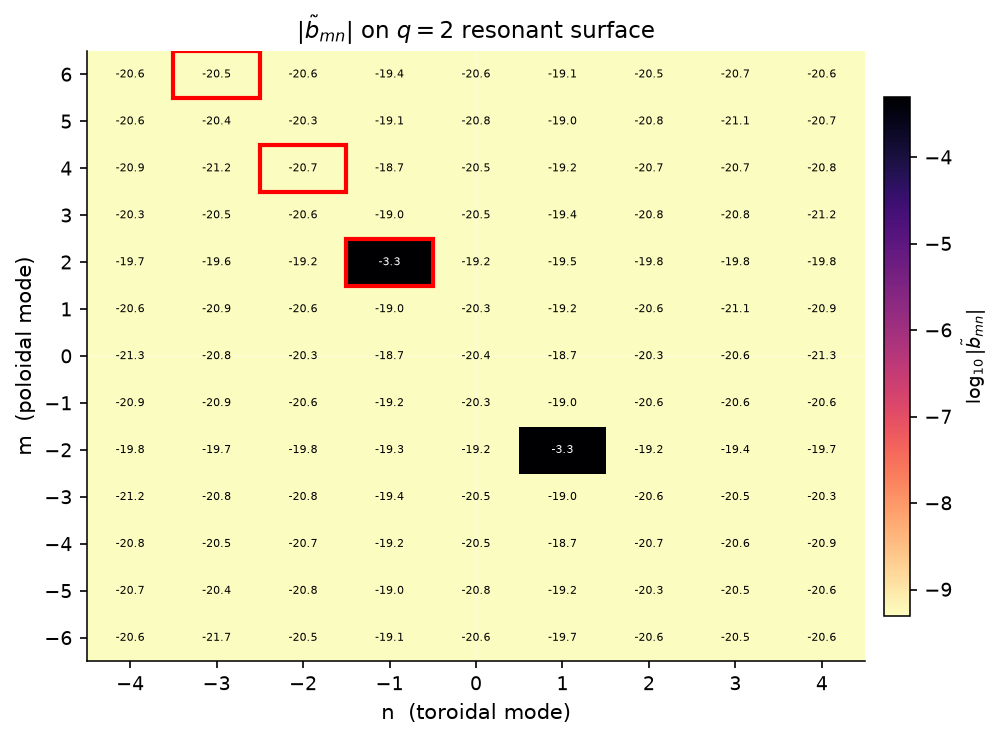
Wir berechnen das vollständige \((m,n)\)-Fourier-Spektrum des divergenzfreien RMP-Templates auf der primären resonanten Fläche. Der resonante Modus \((2,-1)\) und seine getriebenen Harmonischen werden hervorgehoben; der obige Abschnitt zum gemischten Spektrum ist die Begleitansicht, die resonante und nichtresonante Zeilen nach Verstimmung klassifiziert.
[13]:
psi_res_21 = eq.resonant_psi(2, 1)[0]
print(f'Berechne (m,n)-Spektrum auf q=2-Fläche (psi={psi_res_21:.3f}), n_theta=48, n_phi=48...')
b_mn = compute_mn_spectrum(
    delta_B_RMP,
    S=psi_res_21,
    equilibrium=eq,
    m_max=6,
    n_max=4,
    n_theta=48,
    n_phi=48,
)
print(f'Spektrumform: {b_mn.shape}')

fig_sp, ax_sp = plt.subplots(figsize=(7, 5))
plot_mn_heatmap(
    b_mn, m_max=6, n_max=4,
    ax=ax_sp,
    log_scale=True,
    title=r'$|\tilde{b}_{mn}|$ on $q=2$ resonante Fläche',
    cmap='magma_r',
    highlight_Moduss=[(2, -1), (4, -2), (6, -3)],
)
plt.tight_layout()
plt.show()
Berechne (m,n)-Spektrum auf q=2-Fläche (psi=0.167), n_theta=48, n_phi=48...
Spektrumform: (13, 9)
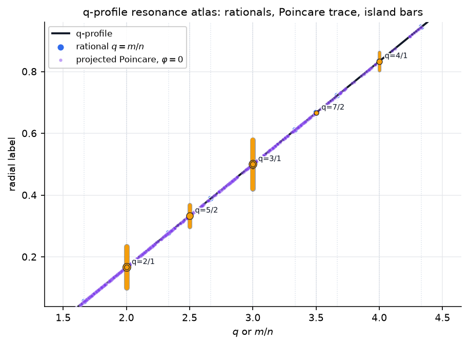
[MAGNETIC_SPECTRUM_ATLAS] Mehrkomponenten-Atlas des \(B^r\)-Spektrums#
Die obige Einzel-Flächen-Heatmap ist nützlich, um eine dominante RMP-Zeile zu prüfen; produktive Analysen magnetischer Topologie benötigen aber meist eine Familienansicht. Hier bauen wir eine divergenzfreie Mehrkomponenten-Störung, berechnen das Nardon-artige kontravariante radiale Spektrum \(\tilde b^1_{mn}=\delta B^1/B_0^3\) auf einem radialen Stack und analysieren alle angeforderten resonanten Zeilen gemeinsam.
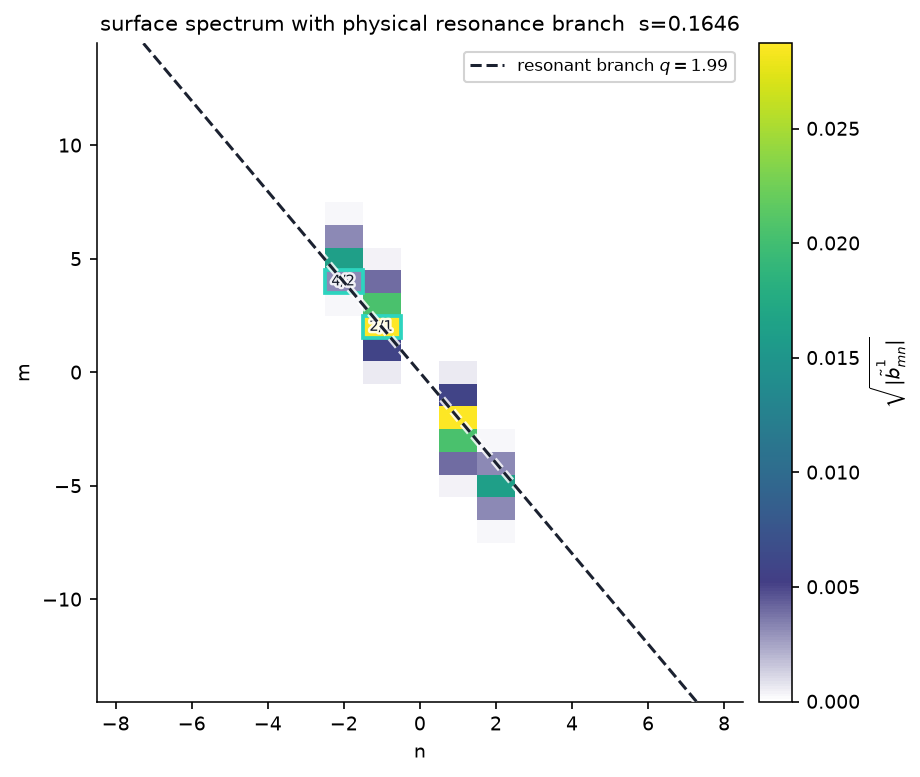
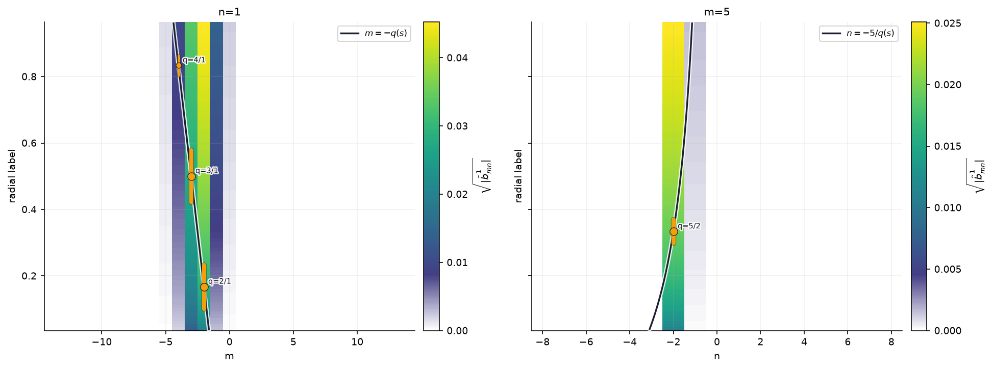
Die folgenden Utilities sind absichtlich modular. Der angezeigte Atlas verwendet ein breiteres vorzeichenbehaftetes Fourier-Fenster, 97 radiale Flächen, amplitude_scale='sqrt' und weiße Masken für Null-/fehlende Zeilen. Die nichtlogarithmische Colormap startet auf derselben weißen Basislinie, sodass nahe-null Koeffizienten nicht künstlich vom maskierten Hintergrund getrennt wirken. Vorzeichenbehaftete Achsen zeigen die tatsächlichen Fourier-Zeilen im berechneten Spektrum: (m,n) ist für
ein reelles Feld konjugiert zu (-m,-n), aber (m,n) und (m,-n) sind unabhängige Zeilen mit entgegengesetzter Helizität, sofern das Störmodell keine zusätzliche Symmetrie erzwingt. amplitude_scale='log10' bleibt nützlich, wenn das Ziel eine strikte Prüfung des Dynamikbereichs statt visueller Mustererkennung ist.
plot_rational_surface_mapkombiniert optional q-Profil, niederordentliche rationale Marker, projizierte Poincaré-Punkte und Inselbreitenbalken in der(m/n, s)-Ebene.plot_spectrum_heatmap(..., renderer='pcolormesh')ist die empfohlene Flächenspektrum-Ansicht; sie kann den physikalisch resonanten Astm=-q n_Füberlagern, ohne den Ast entgegengesetzter Helizität zu zeichnen.plot_spectrum_bar3dliefert eine interaktive Plotly-Figur für Rotation, Zoom und Hover-Inspektion dominanter Zeilen.plot_radial_Modus_heatmap(fixed_n=..., resonant_sign=+1)verfolgt alle \(m\)-Zeilen bei festem Fourier-\(n\) und zeichnet den positiven q-Ast in der negativen \(m\)-Halbebene, \(m=-nq(s)\).plot_radial_Modus_heatmap(fixed_m=..., axis_convention='fourier')verfolgt tatsächliche Fourier-\(n\)-Zeilen und zeichnet den positiven q-Ast \(n=-m/q(s)\); q-Kurve und Inselbreitenbalken bleiben unabhängig umschaltbar.
Gelbe vertikale Balken markieren die Ein-Koeffizienten-Nardon-Halbbreitenschätzung an der niederordentlichen rationalen Fläche; ihre Dicke skaliert mit der Amplitude des resonanten Koeffizienten. Sie sind ein optionales Overlay, nicht Teil der Heatmap selbst. Auf jeder radialen Karte wird nur die physikalisch resonante Kurve gezeichnet. Der Ast entgegengesetzter Helizität ist keine konjugierte Diagnose und wird hier absichtlich nicht gespiegelt. Wenn mehrere Harmonische dieselbe reduzierte rationale Fläche teilen, sollte die echte Inselbreite bei endlicher Amplitude aus dem kombinierten resonanten Hamiltonian berechnet werden; die zeilenweisen Balken sind Diagnosen, nicht diese nichtlinear aufsummierte Breite.
[14]:
delta_B_multi_rmp = compose_magnetic_perturbations(
    radial_rmp_field_template(2, 1, amplitude=5.0e-4, phase=0.00, axis_R=eq.R0),
    radial_rmp_field_template(3, 1, amplitude=2.4e-4, phase=0.55, axis_R=eq.R0),
    radial_rmp_field_template(5, 2, amplitude=1.6e-4, phase=-0.35, axis_R=eq.R0),
)

S_scan = np.linspace(0.04, 0.96, 97)
theta_spec = np.linspace(0.0, 2*np.pi, 160, endpoint=False)
phi_spec = np.linspace(0.0, 2*np.pi, 96, endpoint=False)

theta_grid = theta_spec[None, None, :]
phi_grid = phi_spec[:, None, None]
r_scan = eq.r0 * np.sqrt(S_scan)[None, :, None]
R_stack = eq.R0 + r_scan * np.cos(theta_grid)
Z_stack = r_scan * np.sin(theta_grid)
R_stack = np.repeat(R_stack, phi_spec.size, axis=0)
Z_stack = np.repeat(Z_stack, phi_spec.size, axis=0)
Phi_stack = phi_grid + np.zeros_like(R_stack)

dBR_stack, dBZ_stack, dBphi_stack = delta_B_multi_rmp(R_stack, Z_stack, Phi_stack)
Bphi0_stack = eq.B0 * eq.R0 / np.maximum(R_stack, 1.0e-12)
tilde_b1_grid = nardon_radial_perturbation(
    R_stack,
    Z_stack,
    phi_spec,
    theta_spec,
    dBR_stack,
    dBZ_stack,
    dBphi_stack,
    S_scan,
    denominator_B_phi=Bphi0_stack,
)
magnetic_spectrum = radial_perturbation_Fourier_spectrum(
    tilde_b1_grid,
    theta_spec,
    phi_spec,
    radial_labels=S_scan,
    m_max=14,
    n_max=8,
    min_amplitude=1.0e-14,
)
q_scan = eq.q_of_psi(S_scan)
n_scan = [1, 2, 3]
m_scan = {1: range(1, 9), 2: range(2, 13), 3: range(3, 15)}
chains_multi = analyze_resonant_island_chains_multi_n(
    magnetic_spectrum,
    q_scan,
    n_values=n_scan,
    m_values=m_scan,
    min_b_res=1.0e-8,
)

print(f'Radiales Spektrum: {S_scan.size} Flächen, {magnetic_spectrum.m.size} beibehaltene Fourier-Zeilen über |m|<=14, |n|<=8.')
print(f'Mehrfach-RMP-Analyse fand {len(chains_multi)} Schätzungen resonanter Inselketten.')
print('{:>7} {:>9} {:>9} {:>12} {:>12} {:>10}'.format('(m,n)', 's_res', 'q_res', 'b_res', 'half_width', 'phase'))
for chain in sorted(chains_multi, key=lambda item: item.b_res, reverse=True)[:8]:
    print('({:>2d},{:>1d}) {:>9.4f} {:>9.4f} {:>12.3e} {:>12.3e} {:>9.1f}°'.format(
        chain.m, chain.n, chain.radial_label, chain.q, chain.b_res, chain.half_width, np.degrees(chain.phase)
    ))

review_root = PROJECT_ROOT if PROJECT_ROOT is not None else pathlib.Path.cwd()
review_dir = review_root / 'pyna_output/magnetic_spectrum_review'
review_dir.mkdir(parents=True, exist_ok=True)

poincare_trace = None
if 'R_cross_p0' in globals() and len(R_cross_p0):
    S_p0 = np.clip(((R_cross_p0 - eq.R0)**2 + Z_cross_p0**2) / eq.r0**2, 0.0, 1.0)
    q_p0 = eq.q_of_psi(S_p0)
    poincare_trace = PoincaréRationalTrace(
        ratio=q_p0,
        radial_label=S_p0,
        label=r'projizierter Poincaré, $\varphi=0$',
    )

fig_qmap, ax_qmap, rational_markers = plot_rational_surface_map(
    S_scan,
    q_scan,
    n_values=n_scan,
    m_values=m_scan,
    chains=chains_multi,
    poincare=poincare_trace,
    show_poincare=poincare_trace is not None,
    max_island_bars=12,
    annotate_rationals=False,
    title='q-Profil-Resonanzatlas: rationale Flächen, Poincaré-Spur, Inselbalken',
)
fig_qmap.savefig(review_dir / '01_q_profile_resonance_map.png', dpi=180, bbox_inches='tight', facecolor='white')
plt.show()

surface_index = int(np.argmin(np.abs(S_scan - psi_res_21)))
surface_label = float(S_scan[surface_index])
chains_surface = [chain for chain in chains_multi if abs(chain.radial_label - surface_label) <= 0.08]
fig_surface, ax_surface = plt.subplots(figsize=(6.7, 5.7))
plot_spectrum_heatmap(
    magnetic_spectrum,
    radial_index=surface_index,
    m_values=np.arange(-14, 15),
    n_values=np.arange(-8, 9),
    chains=chains_surface,
    q_value=float(q_scan[surface_index]),
    renderer='pcolormesh',
    amplitude_scale='sqrt',
    mask_zeros=True,
    ax=ax_surface,
    cmap='viridis',
    title='Flächenspektrum mit physikalischem Resonanzast',
)
fig_surface.savefig(review_dir / '02_surface_pcolormesh_atlas.png', dpi=180, bbox_inches='tight', facecolor='white')
plt.show()

fig_bar3d = plot_spectrum_bar3d(
    magnetic_spectrum,
    radial_index=surface_index,
    m_values=np.arange(-10, 11),
    n_values=np.arange(-6, 7),
    amplitude_scale='sqrt',
    range_Modus='nonzero',
    bar_width=0.9,
    z_aspect=0.72,
    title='interaktive 3D-Spektrumbalken',
)
fig_bar3d.write_html(str(review_dir / '04_surface_plotly_bar3d.html'), include_plotlyjs='cdn')
try:
    fig_bar3d.write_image(str(review_dir / '04_surface_plotly_bar3d.png'), width=1040, height=650, scale=2)
except Exception as exc:
    print(f'Statischer Plotly-PNG-Export übersprungen: {exc}')
fig_bar3d.show()

fig_radial, axes_radial = plt.subplots(1, 2, figsize=(13.2, 4.9), sharey=True)
plot_radial_Modus_heatmap(
    magnetic_spectrum,
    fixed_n=1,
    Modus_values=np.arange(-14, 15),
    resonant_sign=1,
    q_profile=q_scan,
    chains=chains_multi,
    renderer='pcolormesh',
    amplitude_scale='sqrt',
    mask_zeros=True,
    ax=axes_radial[0],
    cmap='viridis',
    title='n=1',
)
plot_radial_Modus_heatmap(
    magnetic_spectrum,
    fixed_m=5,
    Modus_values=np.arange(-8, 9),
    axis_convention='fourier',
    q_profile=q_scan,
    chains=chains_multi,
    renderer='pcolormesh',
    amplitude_scale='sqrt',
    mask_zeros=True,
    ax=axes_radial[1],
    cmap='viridis',
    title='m=5',
)
plt.tight_layout()
fig_radial.savefig(review_dir / '03_radial_fixed_n_fixed_m_maps.png', dpi=180, bbox_inches='tight', facecolor='white')
plt.show()
Radiales Spektrum: 97 Flächen, 22 beibehaltene Fourier-Zeilen über |m|<=14, |n|<=8.
Mehrfach-RMP-Analyse fand 7 Schätzungen resonanter Inselketten.
  (m,n)     s_res     q_res        b_res   half_width      phase
( 2,1)    0.1667    2.0000    1.661e-03    6.655e-02       0.6°
( 3,1)    0.5000    3.0000    1.535e-03    7.836e-02      27.6°
( 5,2)    0.3333    2.5000    7.401e-04    3.512e-02     -20.1°
( 4,1)    0.8333    4.0000    1.665e-04    2.980e-02      30.1°
( 6,2)    0.5000    3.0000    6.400e-05    1.131e-02     -20.1°
( 4,2)    0.1667    2.0000    2.132e-05    5.332e-03     -20.1°
( 7,2)    0.6667    3.5000    1.742e-06    2.016e-03     -20.1°
Data type cannot be displayed: application/vnd.plotly.v1+json
[PUBLICATION_FIGURE] Sechs-Panel-Figur mit mehreren phi-Schnitten#
Derselbe Schnitt-Helper skaliert auf ein kompaktes Mehrschnitt-Layout. Die O/X-Marker, O-Punkt-Inselbreitenbalken und lokalen stabilen Äste rotieren mit dem toroidalen Winkel, während das PEST-artige Gitter die Koordinatenbedeutung in jedem Panel sichtbar hält.
[15]:
fig_pub, axes_pub = plot_rmp_resonance_sections(
    all_sections_data,
    phi_sections,
    eq=eq,
    components=components,
    colors=ISLAND_CMAPS,
    ncols=3,
    figsize=(12.0, 7.0),
    point_size=1.6,
    point_alpha=0.42,
    compact=True,
    overlays=('pest_grid', 'poincare', 'resonant_Flächen', 'stable_branches', 'island_width_bars', 'xo'),
    title=(
        'Stellarator RMP resonance: Poincaré points, X/O geometry, '
        'island-width bars, stable branches, and PEST-style grid'
    ),
)

out_path = pathlib.Path('pyna_output/rmp_resonance_publication.png')
out_path.parent.mkdir(exist_ok=True)
fig_pub.savefig(str(out_path), dpi=170, bbox_inches='tight', facecolor='white')
print(f'Publikationsabbildung gespeichert unter {out_path}')
from IPython.display import display
display(fig_pub)
plt.close(fig_pub)
Publikationsabbildung gespeichert unter pyna_output/rmp_resonance_publication.png