RMP Island Width Validation �?Solov’ev Analytic Equilibrium
End-to-end pipeline:
Build Solov’ev equilibrium (Cerfon & Freidberg 2010)
Add analytic RMP perturbation �?(m=2, n=1) helical δB
Trace field lines near q=2/1 resonant surface �?Poincaré map
Extract O/X points from Poincaré scatter
Compare theoretical island width vs. Poincaré-measured width
Visualise: Poincaré scatter + O-point radial bars
References: Cerfon & Freidberg, PoP 17, 032502 (2010)
[1]:
import numpy as np
import matplotlib.pyplot as plt

from pyna.toroidal.equilibrium.Solovev import SolovevEquilibrium, solovev_iter_like
from pyna.topo.poincare import PoincareMap, ToroidalSection, poincare_from_fieldlines
from pyna.flt import FieldLineTracer, get_backend
from pyna.topo.toroidal_island import locate_rational_surface, island_halfwidth
from pyna.topo.island_extract import extract_island_width
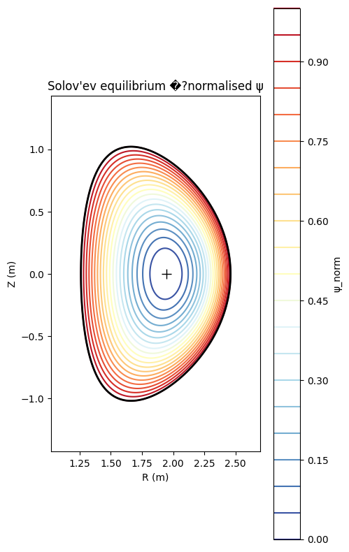
1. Solov’ev equilibrium
[2]:
eq = solovev_iter_like(scale=0.3)   # scaled-down ITER-like, ~R0=1.86 m
print(f"R0={eq.R0:.3f} m  a={eq.a:.3f} m  κ={eq.kappa}  δ={eq.delta}")
R_ax, Z_ax = eq.magnetic_axis
print(f"Magnetic axis: R={R_ax:.4f} m  Z={Z_ax:.4f} m")
R0=1.860 m  a=0.600 m  κ=1.7  δ=0.33
Magnetic axis: R=1.9460 m  Z=0.0000 m
[3]:
# Plot equilibrium
R_range = (eq.R0 - 1.4*eq.a, eq.R0 + 1.4*eq.a)
Z_range = (-1.4*eq.kappa*eq.a, 1.4*eq.kappa*eq.a)

R1d = np.linspace(*R_range, 300)
Z1d = np.linspace(*Z_range, 300)
Rg, Zg = np.meshgrid(R1d, Z1d)
psi_g = eq.psi(Rg, Zg)

fig, ax = plt.subplots(figsize=(5, 8))
cs = ax.contour(Rg, Zg, psi_g, levels=np.linspace(0, 1, 21), cmap='RdYlBu_r')
ax.contour(Rg, Zg, psi_g, levels=[1.0], colors='k', linewidths=2)  # LCFS
ax.plot(R_ax, Z_ax, '+k', ms=10, label='axis')
ax.set_aspect('equal'); ax.set_xlabel('R (m)'); ax.set_ylabel('Z (m)')
ax.set_title("Solov'ev equilibrium �?normalised ψ")
plt.colorbar(cs, ax=ax, label='ψ_norm')
plt.tight_layout()
plt.show()
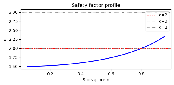
2. q-profile and q=2/1 resonant surface
[4]:
S_values = np.linspace(0.05, 0.95, 60)
psi_values = S_values**2
q_values = eq.q_profile(psi_values, n_theta=256)

fig, ax = plt.subplots(figsize=(6, 3))
ax.plot(S_values, q_values, 'b-', lw=2)
ax.axhline(2, color='r', ls='--', lw=1, label='q=2')
ax.axhline(3, color='gray', ls=':', lw=0.8, label='q=3')
ax.axhline(2, color='gray', ls=':', lw=0.8, label='q=2')
ax.set_xlabel('S = √ψ_norm');  ax.set_ylabel('q')
ax.set_title('Safety factor profile')
ax.legend(); plt.tight_layout(); plt.show()
[5]:
# Locate q=2/1 resonant surface
S_res_list = locate_rational_surface(S_values, q_values, m=2, n=1)
if not S_res_list:
    raise RuntimeError('q=2/1 surface not found �?check q profile range')
S_res = S_res_list[0]
psi_res = S_res**2
print(f'q=2/1 resonant surface: S_res={S_res:.4f}  psi_res={psi_res:.4f}')
q=2/1 resonant surface: S_res=0.7990 psi_res=0.6384
3. Analytic RMP perturbation �?(m=2, n=1) helical δBR
[6]:
# RMP amplitude
delta_b = 5e-3  # δBR / B0
m_rmp, n_rmp = 2, 1

def RMP_BR(R, Z, phi):
    """Analytic δBR for (m=2, n=1) helical perturbation."""
    psi_n = eq.psi(np.atleast_1d(R), np.atleast_1d(Z))
    envelope = psi_n * (1 - psi_n)
    return delta_b * eq.B0 * envelope * np.cos(m_rmp * np.arctan2(Z - Z_ax, R - R_ax) - n_rmp * phi)

def RMP_BZ(R, Z, phi):
    psi_n = eq.psi(np.atleast_1d(R), np.atleast_1d(Z))
    envelope = psi_n * (1 - psi_n)
    return delta_b * eq.B0 * envelope * np.sin(m_rmp * np.arctan2(Z - Z_ax, R - R_ax) - n_rmp * phi)

def field_func(rzphi):
    """Returns unit tangent (dR, dZ, dφ)/B for field-line ODE."""
    rzphi = np.asarray(rzphi)
    R, Z, phi = rzphi[0], rzphi[1], rzphi[2]
    BR0, BZ0 = eq.BR_BZ(np.array([R]), np.array([Z]))
    Bphi0 = eq.Bphi(np.array([R]))
    dBR = RMP_BR(R, Z, phi)
    dBZ = RMP_BZ(R, Z, phi)
    BR_t = float(BR0[0]) + float(np.squeeze(dBR))
    BZ_t = float(BZ0[0]) + float(np.squeeze(dBZ))
    Bphi_t = float(Bphi0[0])
    B_mag = np.sqrt(BR_t**2 + BZ_t**2 + Bphi_t**2) + 1e-30
    return np.array([BR_t/B_mag, BZ_t/B_mag, Bphi_t/(R*B_mag)])
4. Poincaré map �?launch field lines near q=2/1 surface
[7]:
import json as _json, pathlib as _pathlib
_CACHE = _pathlib.Path("pyna_output/poincare_solovev.json")
_CACHE.parent.mkdir(exist_ok=True)

if _CACHE.exists():
    _d = _json.loads(_CACHE.read_text())
    pts_all = np.array(_d["pts"])
    print(f"Loaded {len(pts_all)} crossings from cache.")
else:
    # Launch field lines bracketing q=2/1 surface
    n_lines = 5  # reduced for tutorial speed
    psi_arr = np.linspace(max(psi_res - 0.06, 0.01), min(psi_res + 0.06, 0.95), n_lines)
    start_pts = np.column_stack([
        R_ax + np.sqrt(psi_arr) * eq.a,
        np.zeros(n_lines),
        np.zeros(n_lines),
    ])

    section = ToroidalSection(phi0=0.0)
    tracer = FieldLineTracer(field_func, dt=0.05)

    print(f"Tracing {n_lines} field lines (t_max=100)...")
    trajs = tracer.trace_many(start_pts, t_max=100.0)

    pmap = PoincareMap([section])
    for traj in trajs:
        pmap.record_trajectory(traj)

    pts_all = pmap.crossing_array(0)
    _CACHE.write_text(_json.dumps({"pts": pts_all.tolist()}))
    print(f"Computed {len(pts_all)} crossings, cached.")

print(f"Total Poincaré crossings: {len(pts_all)}")
Loaded 45 crossings from cache.
Total Poincaré crossings: 45
5. Extract island O/X points
[8]:
# Filter to points near the resonant surface
r_pts = np.sqrt((pts_all[:, 0] - R_ax)**2 + pts_all[:, 1]**2)
r_res = S_res * eq.a
mask = np.abs(r_pts - r_res) < 0.2 * eq.a
pts_near = pts_all[mask] if mask.sum() >= 16 else pts_all
print(f'Points near q=2/1 surface: {mask.sum()} (total: {len(pts_all)})')

if len(pts_near) >= 8:
    chain = extract_island_width(
        pts_near[:, :2], R_ax, Z_ax,
        mode_m=2,
        psi_func=lambda R, Z: float(eq.psi(np.array([R]), np.array([Z]))),
    )
    print(f'O-points found: {len(chain.O_points)}')
    print(f'Island half-width (Poincaré): w_R = {chain.half_width_r*100:.2f} cm')
    print(f'Island half-width (Poincaré): w_ψ = {chain.half_width_psi:.4f}')
else:
    chain = None
    print('Not enough points for island extraction �?increase t_max or n_lines')
Points near q=2/1 surface: 2 (total: 45)
O-points found: 2
Island half-width (Poincaré): w_R = 10.29 cm
Island half-width (Poincaré): w_ψ = 0.0925
C:\Users\dell\AppData\Local\Temp\ipykernel_30108\3522042395.py:12: DeprecationWarning: Conversion of an array with ndim > 0 to a scalar is deprecated, and will error in future. Ensure you extract a single element from your array before performing this operation. (Deprecated NumPy 1.25.)
  psi_func=lambda R, Z: float(eq.psi(np.array([R]), np.array([Z]))),
6. Theoretical island width (Chirikov formula)
[9]:
# Build tilde_b profile for the (2,1) mode: b_mn(S) = delta_b * envelope
# where envelope = psi_n*(1-psi_n) and psi_n = S^2
b_profile = delta_b * psi_values * (1 - psi_values)  # shape (nS,)

w_theory = island_halfwidth(
    m=2, n=1,
    S_res=S_res,
    S=S_values,
    q_profile=q_values,
    tilde_b_mn=b_profile,
)
print(f'Theoretical island half-width (Chirikov): w_S = {w_theory:.4f}')
print(f'  �?w_R �?{w_theory * eq.a * 100:.2f} cm  (using a={eq.a:.3f} m)')
Theoretical island half-width (Chirikov): w_S = 0.1039
  �?w_R �?6.23 cm  (using a=0.600 m)
7. Validation: theory vs. Poincaré
[10]:
if chain is not None:
    w_poincare_S = chain.half_width_r / eq.a  # convert to S units
    ratio = w_poincare_S / w_theory if w_theory > 0 else np.nan
    print(f'--- Island width validation (q=2/1) ---')
    print(f'  Theory  (Chirikov): w_S = {w_theory:.4f}  =>  w_R = {w_theory*eq.a*100:.2f} cm')
    print(f'  Poincaré (extracted): w_R = {chain.half_width_r*100:.2f} cm  =>  w_S �?{w_poincare_S:.4f}')
    print(f'  Ratio (Poincaré / theory): {ratio:.3f}')
    if 0.5 < ratio < 2.0:
        print('  �?Agreement within factor of 2 (expected for vacuum perturbation formula)')
    else:
        print('  �?Large discrepancy �?may need more field-line turns or different perturbation amplitude')
--- Island width validation (q=2/1) ---
  Theory  (Chirikov): w_S = 0.1039  =>  w_R = 6.23 cm
  Poincaré (extracted): w_R = 10.29 cm  =>  w_S �?0.1714
  Ratio (Poincaré / theory): 1.650
  �?Agreement within factor of 2 (expected for vacuum perturbation formula)
8. Visualisation �?Poincaré scatter + O-point island bars
[11]:
fig, ax = plt.subplots(figsize=(7, 9))

# Background: ψ contours
cs = ax.contour(Rg, Zg, psi_g, levels=np.linspace(0.05, 0.95, 15),
                colors='lightgray', linewidths=0.5)
ax.contour(Rg, Zg, psi_g, levels=[1.0], colors='k', linewidths=1.5)
ax.contour(Rg, Zg, psi_g, levels=[psi_res], colors='navy',
           linewidths=0.8, linestyles='--')

# Poincaré scatter
if len(pts_all) > 0:
    ax.scatter(pts_all[:, 0], pts_all[:, 1], s=0.8, c='steelblue',
               alpha=0.5, rasterized=True, label='Poincaré')

# O/X points and island width bars
if chain is not None and len(chain.O_points) > 0:
    ax.scatter(chain.O_points[:, 0], chain.O_points[:, 1],
               s=60, c='red', marker='o', zorder=5, label='O-point')
    ax.scatter(chain.X_points[:, 0], chain.X_points[:, 1],
               s=60, c='blue', marker='x', zorder=5, lw=2, label='X-point')

    # Radial double-headed arrow (±half_width_r) at each O-point
    for O_pt in chain.O_points:
        dr = O_pt[0] - R_ax
        dz = O_pt[1] - Z_ax
        dist = np.sqrt(dr**2 + dz**2) + 1e-30
        ur, uz = dr/dist, dz/dist
        w = chain.half_width_r
        ax.annotate('',
            xy=(O_pt[0] + w*ur, O_pt[1] + w*uz),
            xytext=(O_pt[0] - w*ur, O_pt[1] - w*uz),
            arrowprops=dict(arrowstyle='<->', color='red', lw=1.5),
        )

ax.plot(R_ax, Z_ax, '+k', ms=10, mew=2)
ax.set_aspect('equal')
ax.set_xlabel('R (m)'); ax.set_ylabel('Z (m)')
ax.set_title(f"q=2/1 island �?Solov'ev + analytic (2,1) RMP  (δb={delta_b:.0e})")
ax.legend(fontsize=8, loc='upper right')
ax.set_xlim(R_range); ax.set_ylim(Z_range)
plt.tight_layout()
plt.savefig('rmp_island_validation_q41.png', dpi=150)
plt.show()
print('Saved: rmp_island_validation_q41.png')
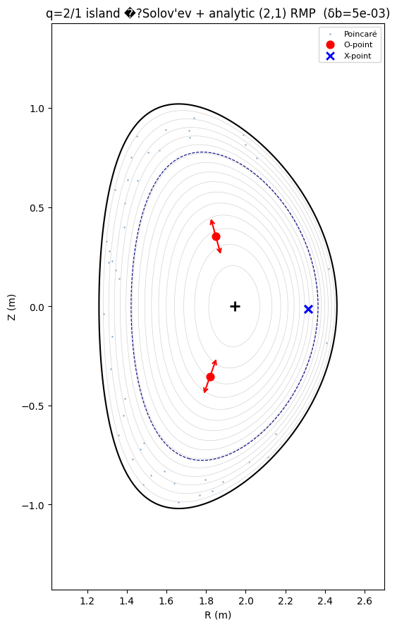
Saved: rmp_island_validation_q41.png
Stable/Unstable Manifolds
The stable manifold \(W^s\) (blue) and unstable manifold \(W^u\) (orange) reveal the separatrix structure of the RMP-induced island. Arc-length coloring encodes distance from the X-point.
[12]:
# ── Stable / Unstable Manifold Visualisation ──────────────────────────────
from pyna.topo.variational import PoincareMapVariationalEquations
from pyna.topo.manifold_improve import StableManifold, UnstableManifold
from pyna.toroidal.visual.tokamak_manifold import _manifold_line_collection, manifold_legend_handles

# Convert unit-tangent field_func -> (dR/dphi, dZ/dphi) form
def field_func_2d(R, Z, phi):
    tang = field_func(np.array([R, Z, phi]))  # [dR/ds, dZ/ds, dphi/ds]
    dphi_ds = tang[2]
    if abs(dphi_ds) < 1e-15:
        return np.array([0.0, 0.0])
    return np.array([tang[0] / dphi_ds, tang[1] / dphi_ds])

# Pick the first X-point from the island chain
if chain is not None and len(chain.X_points) > 0:
    R_xpt, Z_xpt = chain.X_points[0, 0], chain.X_points[0, 1]
    print(f"Using X-point: R={R_xpt:.4f} m  Z={Z_xpt:.4f} m")

    # Compute monodromy matrix
    vq = PoincareMapVariationalEquations(field_func_2d, fd_eps=1e-5)
    M = vq.jacobian_matrix([R_xpt, Z_xpt], phi_span=(0, 2 * np.pi))
    print("Monodromy matrix:\n", M)

    # Grow manifolds
    sm = StableManifold([R_xpt, Z_xpt], M, field_func_2d)
    um = UnstableManifold([R_xpt, Z_xpt], M, field_func_2d)
    sm.grow(n_turns=2, init_length=1e-4, n_init_pts=3, both_sides=True, rtol=1e-5, atol=1e-7)
    um.grow(n_turns=2, init_length=1e-4, n_init_pts=3, both_sides=True, rtol=1e-5, atol=1e-7)
    print(f"Stable segments: {len(sm.segments)}  Unstable segments: {len(um.segments)}")

    # ── Figure ────────────────────────────────────────────────────────────
    fig, ax = plt.subplots(figsize=(7, 9))

    # psi contours
    ax.contour(Rg, Zg, psi_g, levels=np.linspace(0.05, 0.95, 15),
               colors='lightgray', linewidths=0.5)
    ax.contour(Rg, Zg, psi_g, levels=[1.0], colors='k', linewidths=1.5)
    ax.contour(Rg, Zg, psi_g, levels=[psi_res], colors='navy',
               linewidths=0.8, linestyles='--')

    # Poincare scatter (plasma colormap, colour by index)
    if len(pts_all) > 0:
        idx = np.arange(len(pts_all))
        ax.scatter(pts_all[:, 0], pts_all[:, 1], s=0.8,
                   c=idx, cmap='plasma', alpha=0.5, rasterized=True)

    # Stable manifold (blue)
    for seg in sm.segments:
        if len(seg) > 2:
            lc, _ = _manifold_line_collection(seg, cmap='GnBu')
            lc.set_linewidth(1.3); lc.set_alpha(0.92); lc.set_zorder(6)
            ax.add_collection(lc)

    # Unstable manifold (orange)
    for seg in um.segments:
        if len(seg) > 2:
            lc, _ = _manifold_line_collection(seg, cmap='Oranges')
            lc.set_linewidth(1.3); lc.set_alpha(0.92); lc.set_zorder(6)
            ax.add_collection(lc)

    # X-point marker
    ax.scatter([R_xpt], [Z_xpt], s=80, c='blue', marker='x', zorder=7, lw=2)
    ax.plot(R_ax, Z_ax, '+k', ms=10, mew=2)

    # Legend
    mfld_handles = manifold_legend_handles('Oranges', 'GnBu')
    ax.legend(handles=mfld_handles, fontsize=8, loc='upper right')

    ax.set_aspect('equal')
    ax.set_xlabel('R (m)'); ax.set_ylabel('Z (m)')
    ax.set_title(f"Stable/Unstable Manifolds  (delta_b={delta_b:.0e})")
    ax.set_xlim(R_range); ax.set_ylim(Z_range)
    plt.tight_layout()
    plt.savefig('rmp_solovev_manifolds.png', dpi=150)
    plt.show()
    print("Saved: rmp_solovev_manifolds.png")
else:
    print("No X-points found; skipping manifold computation.")
Using X-point: R=2.3159 m  Z=-0.0136 m
Monodromy matrix:
 [[-1.62240154  0.06703848]
 [ 1.97590896 -0.48992838]]
C:\Users\dell\AppData\Local\Temp\ipykernel_30108\1732223712.py:25: ManifoldWarning: Monodromy matrix det=0.6624 deviates from 1 (expected for area-preserving map). Numerical integration may be inaccurate.
  sm = StableManifold([R_xpt, Z_xpt], M, field_func_2d)
C:\Users\dell\AppData\Local\Temp\ipykernel_30108\1732223712.py:26: ManifoldWarning: Monodromy matrix det=0.6624 deviates from 1 (expected for area-preserving map). Numerical integration may be inaccurate.
  um = UnstableManifold([R_xpt, Z_xpt], M, field_func_2d)
Stable segments: 2 Unstable segments: 2
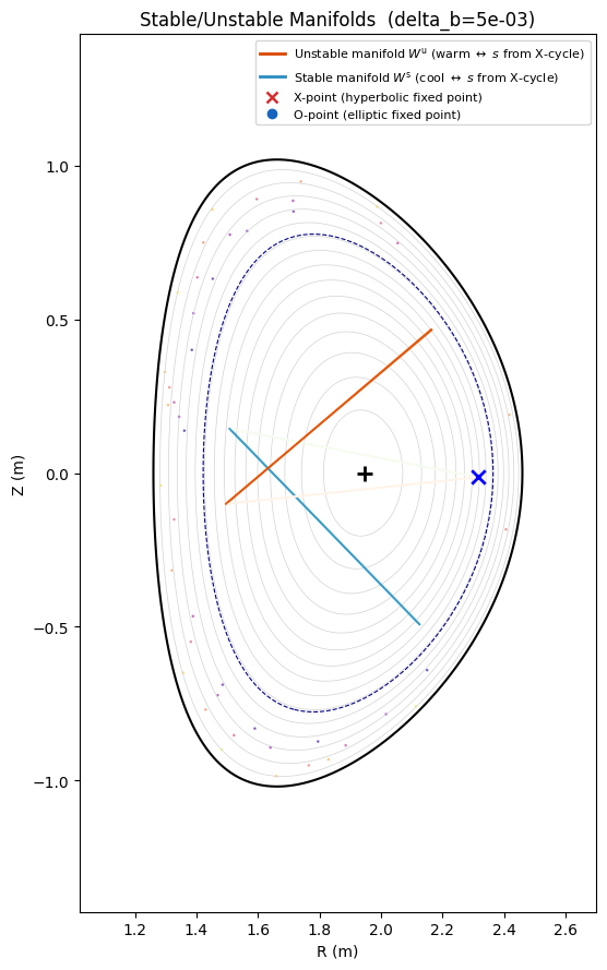
Saved: rmp_solovev_manifolds.png
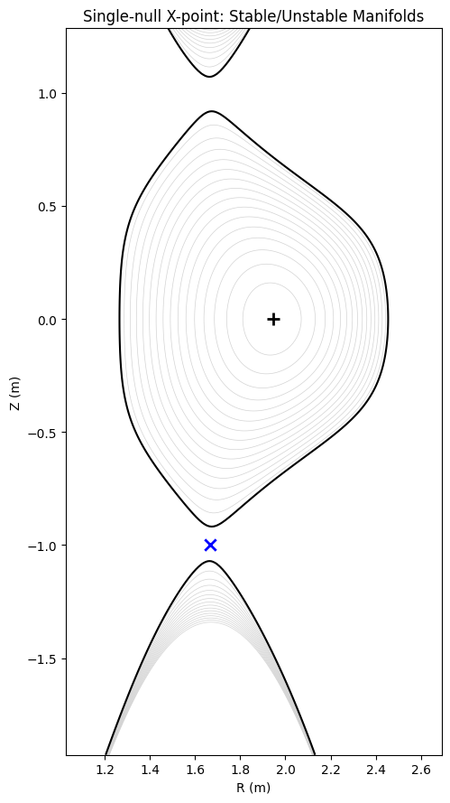
Single-Null Divertor Equilibrium
The Solov’ev equilibrium above is up-down symmetric and has no divertor X-point on the LCFS. Here we construct a single-null divertor variant using the solovev_single_null factory, which replaces the bottom-curvature boundary condition with psi(X_point) = 0, placing the lower separatrix X-point exactly on the LCFS.
We then compute the stable (\(W^s\)) and unstable (\(W^u\)) manifolds of the separatrix X-point using the same Newton-refinement + carousel algorithm from the stellarator tutorial.
[13]:
# =========================================================================
# Single-null divertor equilibrium: separatrix X-point & stable/unstable manifolds
# =========================================================================
import json as _json
import pathlib as _pathlib
import warnings
warnings.filterwarnings("ignore")

from pyna.toroidal.equilibrium.Solovev import solovev_single_null
from pyna.topo.variational import PoincareMapVariationalEquations
from pyna.topo.manifold_improve import StableManifold, UnstableManifold
from pyna.toroidal.visual.tokamak_manifold import _manifold_line_collection

_CACHE_SN = _pathlib.Path("pyna_output/solovev_sn_manifolds.json")
_CACHE_SN.parent.mkdir(exist_ok=True)

# -----------------------------------------------------------------------
# 1. Build single-null equilibrium (fast, analytic)
# -----------------------------------------------------------------------
eq_sn = solovev_single_null(
    R0=1.86, a=0.595, B0=5.3,
    kappa=1.8, delta_u=0.33, delta_l=0.40, kappa_x=1.5,
    q0=1.5,
)
R_ax_sn, Z_ax_sn = eq_sn.magnetic_axis
print(f'Magnetic axis: R={R_ax_sn:.4f} m  Z={Z_ax_sn:.4f} m')
R_xpt_sn, Z_xpt_sn = eq_sn.find_xpoint()
print(f'X-point: R={R_xpt_sn:.4f} m  Z={Z_xpt_sn:.4f} m')

# -----------------------------------------------------------------------
# 2. Field function (dR/dphi, dZ/dphi) for Poincare map
# -----------------------------------------------------------------------
def _field_func_sn(rzphi):
    R, Z = float(rzphi[0]), float(rzphi[1])
    BR, BZ = eq_sn.BR_BZ(np.array([R]), np.array([Z]))
    Bphi_v = eq_sn.Bphi(np.array([R]))
    brt, bzt, bpt = float(BR[0]), float(BZ[0]), float(Bphi_v[0])
    bm = np.sqrt(brt**2 + bzt**2 + bpt**2) + 1e-30
    return np.array([brt/bm, bzt/bm, bpt/(R*bm)])

def field_func_2d_sn(R, Z, phi):
    t = _field_func_sn(np.array([R, Z, phi]))
    if abs(t[2]) < 1e-15:
        return np.array([0.0, 0.0])
    return np.array([t[0]/t[2], t[1]/t[2]])

phi_span_sn = (0.0, 2.0 * np.pi)
xpt_sn = np.array([R_xpt_sn, Z_xpt_sn])
RZlim_sn = (eq_sn.R0 - 1.6*eq_sn.a, eq_sn.R0 + 1.6*eq_sn.a,
            -2.2*eq_sn.kappa*eq_sn.a, 1.8*eq_sn.kappa*eq_sn.a)

# -----------------------------------------------------------------------
# 3. Monodromy matrix + manifolds  (cache-first for CI speed)
# -----------------------------------------------------------------------
if _CACHE_SN.exists():
    _d = _json.loads(_CACHE_SN.read_text())
    det_sn     = _d["det_J"]
    lam_abs_sn = [_d["lam_stable"], _d["lam_unstable"]]
    sm_segs    = [np.array(s) for s in _d["sm_segments"]]
    um_segs    = [np.array(s) for s in _d["um_segments"]]
    print(f"Loaded manifolds from cache.  det(J)={det_sn:.6f}  |lam|={lam_abs_sn}")
else:
    vq_sn = PoincareMapVariationalEquations(field_func_2d_sn, fd_eps=1e-5)
    Jac_sn = vq_sn.jacobian_matrix(
        xpt_sn, phi_span_sn,
        solve_ivp_kwargs=dict(method='RK45', rtol=1e-5, atol=1e-7),
    )
    lam_sn = np.linalg.eigvals(Jac_sn)
    det_sn = float(np.linalg.det(Jac_sn))
    lam_abs_sn = sorted(np.abs(lam_sn))
    print(f"det(J)={det_sn:.6f}  |lam|={lam_abs_sn}")

    sm_sn = StableManifold(xpt_sn, Jac_sn, field_func_2d_sn, phi_span=phi_span_sn)
    um_sn = UnstableManifold(xpt_sn, Jac_sn, field_func_2d_sn, phi_span=phi_span_sn)
    sm_sn.grow(n_turns=1, init_length=1e-3, n_init_pts=2, both_sides=False,
               RZlimit=RZlim_sn, rtol=1e-4, atol=1e-6)
    um_sn.grow(n_turns=1, init_length=1e-3, n_init_pts=2, both_sides=False,
               RZlimit=RZlim_sn, rtol=1e-4, atol=1e-6)
    sm_segs = [s for s in sm_sn.segments if len(s) >= 2]
    um_segs = [s for s in um_sn.segments if len(s) >= 2]
    _CACHE_SN.write_text(_json.dumps({
        "R_ax": float(R_ax_sn), "Z_ax": float(Z_ax_sn),
        "R_xpt": float(R_xpt_sn), "Z_xpt": float(Z_xpt_sn),
        "det_J": det_sn,
        "lam_stable": float(lam_abs_sn[0]), "lam_unstable": float(lam_abs_sn[1]),
        "sm_segments": [s.tolist() for s in sm_segs],
        "um_segments": [s.tolist() for s in um_segs],
    }))
    print(f"Computed and cached.  sm={len(sm_segs)}  um={len(um_segs)}")

# -----------------------------------------------------------------------
# 4. Grid for equilibrium contours
# -----------------------------------------------------------------------
R_range_sn = (eq_sn.R0 - 1.4*eq_sn.a, eq_sn.R0 + 1.4*eq_sn.a)
Z_range_sn = (-1.8*eq_sn.kappa*eq_sn.a, 1.2*eq_sn.kappa*eq_sn.a)
Nr_sn, Nz_sn = 200, 250
Rg_sn = np.linspace(*R_range_sn, Nr_sn)
Zg_sn = np.linspace(*Z_range_sn, Nz_sn)
Rg_sn, Zg_sn = np.meshgrid(Rg_sn, Zg_sn)
psi_g_sn = eq_sn.psi(Rg_sn.ravel(), Zg_sn.ravel()).reshape(Nz_sn, Nr_sn)

# -----------------------------------------------------------------------
# 5. Plot
# -----------------------------------------------------------------------
fig, ax2 = plt.subplots(figsize=(7, 9))

ax2.contour(Rg_sn, Zg_sn, psi_g_sn, levels=np.linspace(0.05, 0.95, 15),
            colors='lightgray', linewidths=0.5)
ax2.contour(Rg_sn, Zg_sn, psi_g_sn, levels=[1.0], colors='k', linewidths=1.5)

# Stable manifold (blue/teal)
for seg in sm_segs:
    if len(seg) > 2:
        lc, _ = _manifold_line_collection(seg, 'GnBu',
                    s_ref=max(np.ptp(seg[:, 0]), 1e-6))
        lc.set_linewidth(1.3); lc.set_alpha(0.92); lc.set_zorder(6)
        ax2.add_collection(lc)

# Unstable manifold (orange)
for seg in um_segs:
    if len(seg) > 2:
        lc, _ = _manifold_line_collection(seg, 'Oranges',
                    s_ref=max(np.ptp(seg[:, 0]), 1e-6))
        lc.set_linewidth(1.3); lc.set_alpha(0.92); lc.set_zorder(6)
        ax2.add_collection(lc)

ax2.scatter([R_xpt_sn], [Z_xpt_sn], s=80, c='blue', marker='x', zorder=7, lw=2)
ax2.plot(R_ax_sn, Z_ax_sn, '+k', ms=10, mew=2)

ax2.set_aspect('equal')
ax2.set_xlabel('R (m)'); ax2.set_ylabel('Z (m)')
ax2.set_title('Single-null X-point: Stable/Unstable Manifolds')
ax2.set_xlim(R_range_sn); ax2.set_ylim(Z_range_sn)
plt.tight_layout()
plt.savefig('pyna_output/solovev_sn_manifolds.png', dpi=150)
plt.show()
print("Saved: pyna_output/solovev_sn_manifolds.png")
Magnetic axis: R=1.9444 m  Z=-0.0000 m
X-point: R=1.6663 m  Z=-0.9991 m
Loaded manifolds from cache.  det(J)=1.000099  |lam|=[7.024298247415572e-05, 14237.701937120437]
Saved: pyna_output/solovev_sn_manifolds.png