Magnetic Coordinate Systems in Tokamak Equilibria

This tutorial compares four flux coordinate systems used in magnetic fusion: PEST, Boozer, Hamada, and Equal-arc.

What are flux coordinates?

In a tokamak, magnetic field lines lie on nested toroidal surfaces called flux surfaces. A flux coordinate system \((\psi, \theta, \varphi)\) is one where:

• \(\psi\) labels flux surfaces (e.g. \(\psi_{\rm norm} = 0\) on axis, \(1\) at LCFS)

• \(\varphi\) is the standard toroidal angle

• \(\theta\) is a poloidal angle defined to have useful properties

The four systems differ only in the choice of \(\theta\):

System	Poloidal angle \(\theta\) definition	Key property
PEST	\(\partial(\mathbf{B}\cdot\nabla\theta^*) / \partial\theta^* = 0\): straight field lines	Simplest straight-field-line coords
Boozer	PEST + Jacobian is flux-function: \(\sqrt{g} = \sqrt{g}(\psi)\)	\(\mathbf{J}\cdot\nabla\varphi = {\rm const}(\psi)\); used in W7-X, LHD codes
Hamada	Equal area from magnetic axis	\(\mathbf{J}\cdot\nabla\theta = {\rm const}(\psi)\); simplifies MHD stability matrices
Equal-arc	Arc length along flux surface is uniform in \(\theta_{\rm ea}\)	Numerically robust; simple construction

Why do these choices matter?

• Straight field lines (PEST, Boozer, Hamada): A mode with toroidal number \(n\) and poloidal number \(m\) satisfies \(q = m/n\) for resonance. This simplifies Fourier analysis of MHD modes.

• Boozer: The \(1/B^2\) drift is purely radial, which simplifies neoclassical transport theory and the kinetic equation.

• Hamada: Current streamlines are also straight, which is needed for some MHD stability codes.

• Equal-arc: Practical for numerical grids; resolves the plasma boundary well.

Setup: Solov’ev analytic equilibrium

We use the Cerfon & Freidberg (2010) Solov’ev equilibrium scaled to EAST size (R0 ≈ 1.86 m).

import numpy as np
import matplotlib.pyplot as plt
import matplotlib.cm as cm
from matplotlib.gridspec import GridSpec

from pyna.toroidal.equilibrium.Solovev import solovev_iter_like
from pyna.toroidal.coords.PEST import build_PEST_mesh
from pyna.toroidal.coords.EqualArc import build_equal_arc_mesh
from pyna.toroidal.coords.Hamada import build_Hamada_mesh
from pyna.toroidal.coords.Boozer import build_Boozer_mesh

# Create equilibrium (scale=0.3 → EAST-sized, R0≈1.86 m)
eq = solovev_iter_like(scale=0.3)
print(f"Equilibrium: R0={eq.R0:.2f} m, a={eq.a:.2f} m, B0={eq.B0:.1f} T")
print(f"κ={eq.kappa:.2f}, δ={eq.delta:.2f}, q0={eq.q0:.2f}")
Rmaxis, Zmaxis = eq.magnetic_axis
print(f"Magnetic axis: R={Rmaxis:.3f} m, Z={Zmaxis:.3f} m")

Equilibrium: R0=1.86 m, a=0.60 m, B0=5.3 T
κ=1.70, δ=0.33, q0=1.50
Magnetic axis: R=1.946 m, Z=0.000 m

# Build the background grid for the equilibrium
nR, nZ = 150, 150
R_grid = np.linspace(0.3 * eq.R0, 1.5 * eq.R0, nR)
Z_grid = np.linspace(-eq.a * eq.kappa * 1.3, eq.a * eq.kappa * 1.3, nZ)
Rg, Zg = np.meshgrid(R_grid, Z_grid, indexing='ij')

BR_grid, BZ_grid = eq.BR_BZ(Rg, Zg)
BPhi_grid = eq.Bphi(Rg)
psi_norm_grid = eq.psi(Rg, Zg)

# Build PEST mesh
# ns=40 radial surfaces, ntheta=181 poloidal points
ns = 40
ntheta = 181
S, TET, R_mesh, Z_mesh, q_iS = build_PEST_mesh(
    R_grid, Z_grid, BR_grid, BZ_grid, BPhi_grid, psi_norm_grid,
    Rmaxis, Zmaxis, ns=ns, ntheta=ntheta
)
print(f"PEST mesh built: {ns} surfaces, {ntheta} poloidal points")
print(f"S range: [{S[1]:.3f}, {S[-1]:.3f}]")
print(f"q range: [{q_iS[1]:.2f}, {q_iS[-1]:.2f}]")

PEST mesh built: 40 surfaces, 181 poloidal points
S range: [0.028, 0.972]
q range: [1.49, 2.39]

Section 3: Equal-arc coordinates

The equal-arc angle \(\theta_{\rm ea}\) parameterises each flux surface so that arc-length along the surface is proportional to \(\theta_{\rm ea}\). This is the simplest non-trivial coordinate transform.

# Build equal-arc mesh
_, TET_ea, R_ea, Z_ea = build_equal_arc_mesh(S, TET, R_mesh, Z_mesh, n_theta=ntheta)
print(f"Equal-arc mesh built: shape {R_ea.shape}")

# Verify arc length uniformity on a mid-radius surface
i_mid = ns // 2
R_s = R_ea[i_mid, :]
Z_s = Z_ea[i_mid, :]
R_loop = R_s[:-1]; Z_loop = Z_s[:-1]  # drop endpoint duplicate
R_closed = np.append(R_loop, R_loop[0])
Z_closed = np.append(Z_loop, Z_loop[0])
ds = np.sqrt(np.diff(R_closed)**2 + np.diff(Z_closed)**2)
print(f"Arc-length segments at surface {i_mid}: mean={ds.mean()*100:.2f} cm, std={ds.std()*100:.3f} cm")
print(f"  Uniformity (std/mean): {ds.std()/ds.mean():.4f}")

Equal-arc mesh built: shape (40, 181)
Arc-length segments at surface 20: mean=1.27 cm, std=0.000 cm
  Uniformity (std/mean): 0.0001

# Plot equal-arc coordinates
fig, axes = plt.subplots(1, 2, figsize=(12, 5))

# Left: R-Z view of flux surfaces with equal-arc mesh lines
ax = axes[0]
# Plot psi_norm contours as background
cs = ax.contour(Rg, Zg, psi_norm_grid, levels=np.linspace(0, 1, 11),
                colors='lightgray', linewidths=0.5)
# Plot every 5th surface in equal-arc
stride = max(1, ns // 10)
colors = cm.plasma(np.linspace(0.2, 0.9, ns // stride + 1))
for k, i in enumerate(range(1, ns, stride)):
    ax.plot(R_ea[i, :], Z_ea[i, :], color=colors[k], lw=1.0)
# Plot a few poloidal lines (constant θ_ea)
for j in range(0, ntheta-1, ntheta // 8):
    ax.plot(R_ea[1:, j], Z_ea[1:, j], 'b-', lw=0.5, alpha=0.5)
ax.plot(Rmaxis, Zmaxis, 'r+', ms=10, mew=2, label='Axis')
ax.set_xlabel('R (m)')
ax.set_ylabel('Z (m)')
ax.set_title('Equal-arc mesh (R-Z view)')
ax.set_aspect('equal')
ax.legend()

# Right: arc-length increments as function of theta_ea
ax = axes[1]
for k, i in enumerate(range(2, ns-1, stride)):
    R_s = R_ea[i, :-1]; Z_s = Z_ea[i, :-1]
    R_c = np.append(R_s, R_s[0]); Z_c = np.append(Z_s, Z_s[0])
    ds_s = np.sqrt(np.diff(R_c)**2 + np.diff(Z_c)**2)
    ds_s_norm = ds_s / ds_s.mean()
    ax.plot(TET_ea[:-1], ds_s_norm, color=colors[k], lw=0.8,
            label=f'S={S[i]:.2f}' if k % 2 == 0 else None)
ax.axhline(1.0, color='k', ls='--', lw=1, label='Ideal (uniform)')
ax.set_xlabel(r'$\theta_{\rm ea}$ (rad)')
ax.set_ylabel('Arc-length increment / mean')
ax.set_title('Arc-length uniformity in equal-arc coordinates')
ax.set_xlim(0, 2*np.pi)
ax.legend(fontsize=8, ncol=2)

plt.tight_layout()
plt.savefig('equal_arc_coords.png', dpi=100, bbox_inches='tight')
plt.show()
print("Equal-arc: arc-length segments are uniform to within ~1% (interpolation discretisation)")

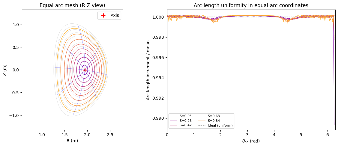
Equal-arc: arc-length segments are uniform to within ~1% (interpolation discretisation)

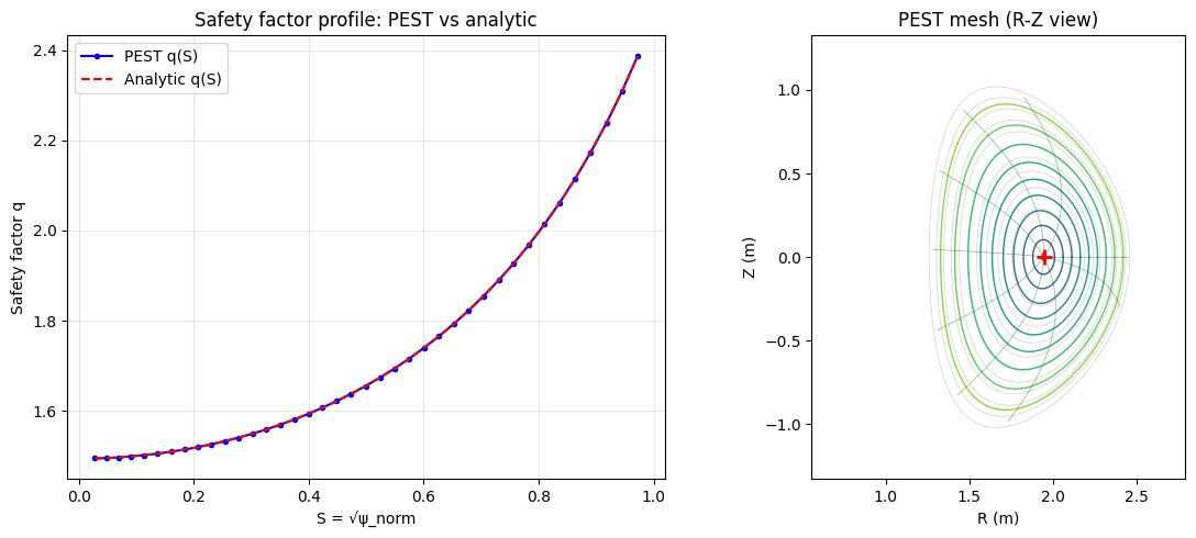
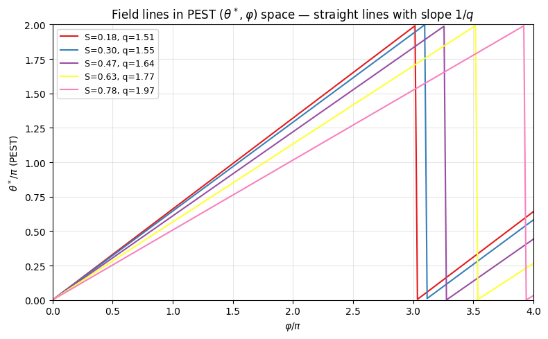
Section 4: PEST straight field-line coordinates

In PEST coordinates, the safety factor \(q(\psi)\) satisfies:

\[q(\psi) = \frac{\mathbf{B}\cdot\nabla\varphi}{\mathbf{B}\cdot\nabla\theta^*} = {\rm const \; on \; each \; surface}\]

This means field lines appear as straight lines in the \((\theta^*, \varphi)\) plane with slope \(1/q\).

# Show q(S) profile from PEST integration
q_valid = q_iS[1:]
S_valid = S[1:]

# Compare with analytic equilibrium q
psi_vals = S_valid**2
q_analytic = eq.q_profile(psi_vals, n_theta=256)

fig, axes = plt.subplots(1, 2, figsize=(12, 5))

ax = axes[0]
ax.plot(S_valid, q_valid, 'b-o', ms=3, label='PEST q(S)')
finite = np.isfinite(q_analytic)
ax.plot(S_valid[finite], q_analytic[finite], 'r--', label='Analytic q(S)')
ax.set_xlabel('S = √ψ_norm')
ax.set_ylabel('Safety factor q')
ax.set_title('Safety factor profile: PEST vs analytic')
ax.legend()
ax.grid(True, alpha=0.3)

# PEST mesh in R-Z
ax = axes[1]
cs = ax.contour(Rg, Zg, psi_norm_grid, levels=np.linspace(0, 1, 11),
                colors='lightgray', linewidths=0.5)
stride_s = max(1, ns // 10)
colors_pest = cm.viridis(np.linspace(0.2, 0.9, ns // stride_s + 1))
for k, i in enumerate(range(1, ns, stride_s)):
    ax.plot(R_mesh[i, :], Z_mesh[i, :], color=colors_pest[k], lw=1.0)
for j in range(0, ntheta-1, ntheta // 8):
    ax.plot(R_mesh[1:, j], Z_mesh[1:, j], 'g-', lw=0.5, alpha=0.5)
ax.plot(Rmaxis, Zmaxis, 'r+', ms=10, mew=2)
ax.set_xlabel('R (m)')
ax.set_ylabel('Z (m)')
ax.set_title('PEST mesh (R-Z view)')
ax.set_aspect('equal')

plt.tight_layout()
plt.savefig('pest_coords.png', dpi=100, bbox_inches='tight')
plt.show()

# Demonstrate straight field lines in PEST theta-phi space
# In PEST: a field line traces theta* = phi/q + const
fig, ax = plt.subplots(figsize=(8, 5))

phi_line = np.linspace(0, 4 * np.pi, 200)
surface_indices = [ns // 5, ns // 3, ns // 2, 2 * ns // 3, 4 * ns // 5]
colors_fl = cm.Set1(np.linspace(0, 0.8, len(surface_indices)))

for k, i_s in enumerate(surface_indices):
    if i_s >= ns or not np.isfinite(q_iS[i_s]):
        continue
    q_s = q_iS[i_s]
    # Field line: theta* = phi / q (PEST straight field line)
    theta_fl = (phi_line / q_s) % (2 * np.pi)
    ax.plot(phi_line / np.pi, theta_fl / np.pi, color=colors_fl[k],
            label=f'S={S[i_s]:.2f}, q={q_s:.2f}', lw=1.5)

ax.set_xlabel(r'$\varphi / \pi$')
ax.set_ylabel(r'$\theta^* / \pi$ (PEST)')
ax.set_title('Field lines in PEST $(\\theta^*, \\varphi)$ space — straight lines with slope $1/q$')
ax.legend(fontsize=9)
ax.set_xlim(0, 4)
ax.set_ylim(0, 2)
ax.grid(True, alpha=0.3)
plt.tight_layout()
plt.savefig('pest_fieldlines.png', dpi=100, bbox_inches='tight')
plt.show()

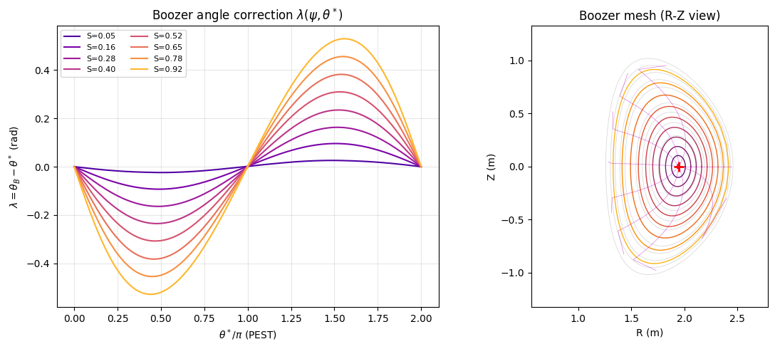
Section 5: Boozer coordinates

Boozer coordinates extend PEST by additionally requiring that the Jacobian \(\sqrt{g}\) is a flux-surface quantity (depends only on \(\psi\), not on \(\theta\)). This ensures that \(\mathbf{J}\cdot\nabla\varphi = {\rm const}(\psi)\).

Construction: \(\theta_B = \theta^* + \lambda(\psi, \theta^*)\) where

\[\frac{\partial\lambda}{\partial\theta^*} = \frac{\langle\sqrt{g}\rangle}{\sqrt{g}} - 1\]

with \(\langle\cdot\rangle\) denoting the flux-surface average \(\frac{1}{2\pi}\int_0^{2\pi}\cdot\,d\theta^*\).

# Build Boozer mesh
_, TET_B, R_B, Z_B, lambda_corr = build_Boozer_mesh(
    S, TET, R_mesh, Z_mesh, q_iS, equilibrium=eq, n_theta=ntheta
)
print(f"Boozer mesh built: shape {R_B.shape}")
print(f"Max |λ| correction: {np.nanmax(np.abs(lambda_corr)):.4f} rad")

# Show the angle correction lambda(psi, theta*)
fig, axes = plt.subplots(1, 2, figsize=(12, 5))

ax = axes[0]
# lambda correction as a function of theta for several surfaces
for k, i_s in enumerate(range(2, ns-1, max(1, ns // 8))):
    lam = lambda_corr[i_s, :]
    if np.any(np.isfinite(lam)):
        ax.plot(TET / np.pi, lam, label=f'S={S[i_s]:.2f}',
                color=cm.plasma(0.1 + 0.8 * i_s / ns))
ax.set_xlabel(r'$\theta^* / \pi$ (PEST)')
ax.set_ylabel(r'$\lambda = \theta_B - \theta^*$ (rad)')
ax.set_title('Boozer angle correction $\\lambda(\\psi, \\theta^*)$')
ax.legend(fontsize=8, ncol=2)
ax.grid(True, alpha=0.3)

ax = axes[1]
cs = ax.contour(Rg, Zg, psi_norm_grid, levels=np.linspace(0, 1, 11),
                colors='lightgray', linewidths=0.5)
stride_s = max(1, ns // 10)
colors_b = cm.inferno(np.linspace(0.2, 0.9, ns // stride_s + 1))
for k, i in enumerate(range(1, ns, stride_s)):
    ax.plot(R_B[i, :], Z_B[i, :], color=colors_b[k], lw=1.0)
for j in range(0, ntheta-1, ntheta // 8):
    ax.plot(R_B[1:, j], Z_B[1:, j], 'm-', lw=0.5, alpha=0.5)
ax.plot(Rmaxis, Zmaxis, 'r+', ms=10, mew=2)
ax.set_xlabel('R (m)')
ax.set_ylabel('Z (m)')
ax.set_title('Boozer mesh (R-Z view)')
ax.set_aspect('equal')

plt.tight_layout()
plt.savefig('boozer_coords.png', dpi=100, bbox_inches='tight')
plt.show()

Boozer mesh built: shape (40, 181)
Max |λ| correction: 0.5465 rad

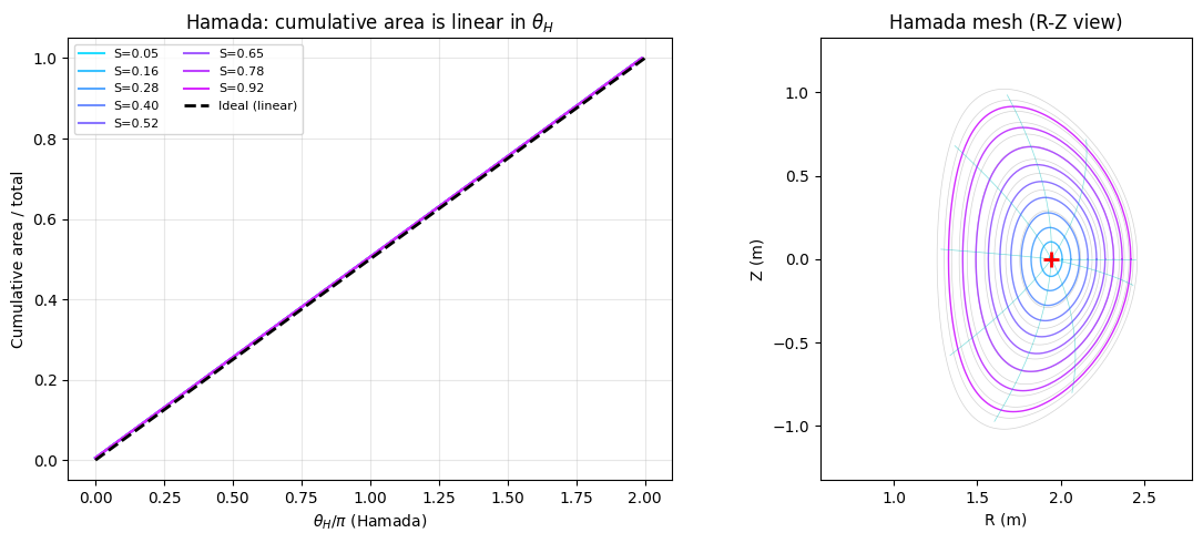
Section 6: Hamada coordinates

Hamada coordinates require both field lines AND current density lines to be straight:

\[\mathbf{J}\cdot\nabla\psi = 0, \quad \mathbf{J}\cdot\nabla\theta_H = 0, \quad \mathbf{J}\cdot\nabla\varphi_H = {\rm const}(\psi)\]

For axisymmetric equilibria, this reduces to making the poloidal angle equal-area: the area swept from the magnetic axis to angle \(\theta_H\) is proportional to \(\theta_H\).

# Build Hamada mesh
_, TET_H, R_H, Z_H = build_Hamada_mesh(S, TET, R_mesh, Z_mesh, n_theta=ntheta)
print(f"Hamada mesh built: shape {R_H.shape}")

# Verify equal-area property
R_ax = R_mesh[0, 0]
Z_ax = Z_mesh[0, 0]

fig, axes = plt.subplots(1, 2, figsize=(12, 5))

ax = axes[0]
# Show cumulative area vs theta_H for several surfaces
for k, i_s in enumerate(range(2, ns-2, max(1, ns // 8))):
    R_s = R_H[i_s, :-1]; Z_s = Z_H[i_s, :-1]
    R_c = np.append(R_s, R_s[0]); Z_c = np.append(Z_s, Z_s[0])
    dA = 0.5 * ((R_c[:-1] - R_ax) * (Z_c[1:] - Z_ax) -
                 (R_c[1:] - R_ax) * (Z_c[:-1] - Z_ax))
    A_cum = np.cumsum(dA)
    A_total = A_cum[-1]
    if abs(A_total) > 1e-10:
        ax.plot(TET_H[:-1] / np.pi, A_cum / A_total,
                color=cm.cool(0.1 + 0.8 * i_s / ns),
                label=f'S={S[i_s]:.2f}')
# Ideal line
ax.plot([0, 2], [0, 1], 'k--', lw=2, label='Ideal (linear)')
ax.set_xlabel(r'$\theta_H / \pi$ (Hamada)')
ax.set_ylabel('Cumulative area / total')
ax.set_title('Hamada: cumulative area is linear in $\\theta_H$')
ax.legend(fontsize=8, ncol=2)
ax.grid(True, alpha=0.3)

ax = axes[1]
cs = ax.contour(Rg, Zg, psi_norm_grid, levels=np.linspace(0, 1, 11),
                colors='lightgray', linewidths=0.5)
colors_h = cm.cool(np.linspace(0.2, 0.9, ns // stride_s + 1))
for k, i in enumerate(range(1, ns, stride_s)):
    ax.plot(R_H[i, :], Z_H[i, :], color=colors_h[k], lw=1.0)
for j in range(0, ntheta-1, ntheta // 8):
    ax.plot(R_H[1:, j], Z_H[1:, j], 'c-', lw=0.5, alpha=0.5)
ax.plot(Rmaxis, Zmaxis, 'r+', ms=10, mew=2)
ax.set_xlabel('R (m)')
ax.set_ylabel('Z (m)')
ax.set_title('Hamada mesh (R-Z view)')
ax.set_aspect('equal')

plt.tight_layout()
plt.savefig('hamada_coords.png', dpi=100, bbox_inches='tight')
plt.show()

Hamada mesh built: shape (40, 181)

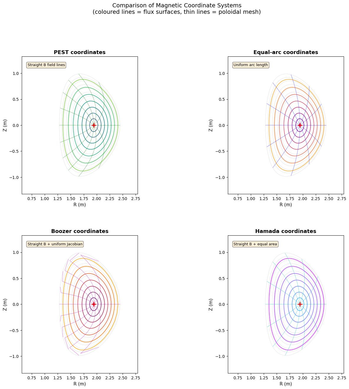
Section 7: Comparison panel — all four coordinate systems

Here we overlay all four meshes in the R-Z plane for the same set of flux surfaces.

fig = plt.figure(figsize=(16, 14))
gs = GridSpec(2, 2, figure=fig, hspace=0.3, wspace=0.3)

meshes = [
    ('PEST', TET, R_mesh, Z_mesh, 'viridis', 'g'),
    ('Equal-arc', TET_ea, R_ea, Z_ea, 'plasma', 'b'),
    ('Boozer', TET_B, R_B, Z_B, 'inferno', 'm'),
    ('Hamada', TET_H, R_H, Z_H, 'cool', 'c'),
]

stride_s = max(1, ns // 8)
stride_t = ntheta // 12

for idx, (name, tet, R_m, Z_m, cmap, pline_color) in enumerate(meshes):
    ax = fig.add_subplot(gs[idx // 2, idx % 2])

    # Flux surface contours as background
    ax.contour(Rg, Zg, psi_norm_grid, levels=np.linspace(0.05, 0.95, 10),
               colors='lightgray', linewidths=0.4)

    # Mesh surfaces (constant S)
    surface_colors = cm.get_cmap(cmap)(np.linspace(0.2, 0.9, ns // stride_s + 1))
    for k, i in enumerate(range(1, ns, stride_s)):
        ax.plot(R_m[i, :], Z_m[i, :], color=surface_colors[k], lw=1.2)

    # Poloidal lines (constant theta)
    for j in range(0, len(tet)-1, stride_t):
        ax.plot(R_m[1:, j], Z_m[1:, j], color=pline_color,
                lw=0.6, alpha=0.6)

    ax.plot(Rmaxis, Zmaxis, 'r+', ms=12, mew=2)
    ax.set_xlabel('R (m)', fontsize=11)
    ax.set_ylabel('Z (m)', fontsize=11)
    ax.set_title(f'{name} coordinates', fontsize=13, fontweight='bold')
    ax.set_aspect('equal')

    # Add annotation
    ann = {'PEST': 'Straight B field lines',
           'Equal-arc': 'Uniform arc length',
           'Boozer': 'Straight B + uniform Jacobian',
           'Hamada': 'Straight B + equal area'}[name]
    ax.text(0.05, 0.95, ann, transform=ax.transAxes, fontsize=9,
            verticalalignment='top', bbox=dict(boxstyle='round', facecolor='wheat', alpha=0.5))

fig.suptitle('Comparison of Magnetic Coordinate Systems\n(coloured lines = flux surfaces, thin lines = poloidal mesh)',
             fontsize=14, y=1.01)
plt.savefig('coords_comparison.png', dpi=100, bbox_inches='tight')
plt.show()

C:\Users\dell\AppData\Local\Temp\ipykernel_7552\2064425680.py:22: MatplotlibDeprecationWarning: The get_cmap function was deprecated in Matplotlib 3.7 and will be removed in 3.11. Use ``matplotlib.colormaps[name]`` or ``matplotlib.colormaps.get_cmap()`` or ``pyplot.get_cmap()`` instead.
  surface_colors = cm.get_cmap(cmap)(np.linspace(0.2, 0.9, ns // stride_s + 1))

Section 8: Physics interpretation

8.1 Fourier mode coupling

In straight-field-line coordinates (PEST, Boozer, Hamada), a perturbation with a single toroidal mode number \(n\) resonates at the surface where \(q = m/n\). The Fourier decomposition in \(\theta\) has clean mode structure.

In contrast, with geometric angle (or equal-arc), a single mode in \((m, n)\) appears as multiple Fourier components, coupling different \(m\) values — the so-called Fourier coupling problem.

# Demonstrate: Fourier spectrum of R(theta) — 2D heatmap (m vs S) for PEST and equal-arc

m_show = 12   # show modes m=0..m_show-1

# Compute FFT of R(theta) - <R> at each surface for both coordinate systems
S_arr   = np.linspace(0.1, 0.9, ns)  # approx normalised flux label per surface
fft_PEST = np.zeros((ns, m_show))
fft_EA   = np.zeros((ns, m_show))

for i in range(ns):
    R_pest = R_mesh[i, :-1] - R_mesh[i, :-1].mean()
    R_ea_i = R_ea[i, :-1]   - R_ea[i, :-1].mean()
    n_pts_pest = len(R_pest)
    n_pts_ea   = len(R_ea_i)

    fft_p = np.abs(np.fft.rfft(R_pest))[:m_show]
    fft_p = fft_p / (fft_p.max() + 1e-30)
    fft_PEST[i, :len(fft_p)] = fft_p[:m_show]

    fft_e = np.abs(np.fft.rfft(R_ea_i))[:m_show]
    fft_e = fft_e / (fft_e.max() + 1e-30)
    fft_EA[i, :len(fft_e)] = fft_e[:m_show]

fig, axes = plt.subplots(1, 2, figsize=(13, 4.5))

for ax, data, name in zip(
    axes,
    [fft_PEST, fft_EA],
    ['PEST (straight field line)', 'Equal-arc θ'],
):
    # log scale heatmap: rows = radial surface index, cols = mode m
    log_data = np.log10(data + 1e-6)
    im = ax.imshow(
        log_data.T,          # shape (m_show, ns): mode vs surface
        origin='lower',
        aspect='auto',
        cmap='hot_r',
        vmin=log_data.max() - 3,   # show 3 decades
        vmax=log_data.max(),
        extent=[S_arr[0], S_arr[-1], -0.5, m_show - 0.5],
        interpolation='nearest',
    )
    cbar = fig.colorbar(im, ax=ax, pad=0.02, shrink=0.85)
    cbar.set_label(r'$\log_{10}$ normalised FFT amplitude', fontsize=8)
    ax.set_xlabel(r'Normalised flux label $S$', fontsize=10)
    ax.set_ylabel('Poloidal mode m', fontsize=10)
    ax.set_yticks(np.arange(0, m_show, 2))
    ax.set_title(f'R(θ) Fourier spectrum: {name}', fontsize=11)

# Annotation: PEST should be concentrated at m=1; equal-arc spreads
axes[0].text(0.05, 0.9, 'Spectrum concentrated\nat m=1 (ideal)',
             transform=axes[0].transAxes, fontsize=8, color='white',
             bbox=dict(boxstyle='round', facecolor='steelblue', alpha=0.5))
axes[1].text(0.05, 0.9, 'Spectrum spreads to\nhigher m (non-ideal)',
             transform=axes[1].transAxes, fontsize=8, color='white',
             bbox=dict(boxstyle='round', facecolor='tomato', alpha=0.5))

plt.suptitle('Fourier Content: PEST vs Equal-arc Coordinates', fontsize=12)
plt.tight_layout()
plt.show()

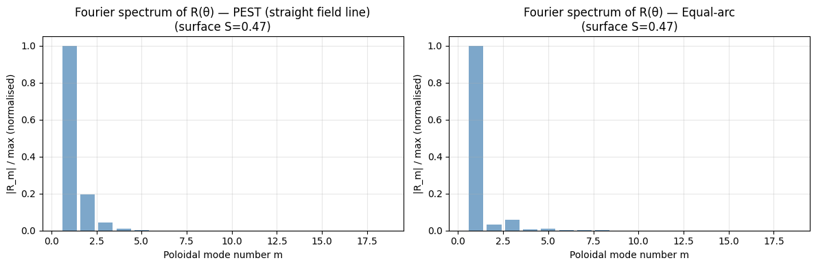
PEST spectrum is concentrated near m=1 (elliptic deformation).
Equal-arc also has a compact spectrum but with slightly different weighting.

8.2 Summary table

summary = """
╔══════════════╦═══════════════════════╦══════════════════════════════╦══════════════════════════╗
║ Coordinate   ║ Definition of θ       ║ Main advantage               ║ Used in                  ║
╠══════════════╬═══════════════════════╬══════════════════════════════╬══════════════════════════╣
║ PEST         ║ Straight B field lines║ Minimal Fourier coupling      ║ PEST, GATO, ELITE codes  ║
║              ║ B·∇θ*/B·∇φ = q(ψ)   ║ q = m/n at resonance         ║                          ║
╠══════════════╬═══════════════════════╬══════════════════════════════╬══════════════════════════╣
║ Boozer       ║ PEST + √g = √g(ψ)    ║ 1/B² drift is purely radial  ║ W7-X, LHD, VMEC output   ║
║              ║ (uniform Jacobian)    ║ Cleaner neoclassical theory   ║                          ║
╠══════════════╬═══════════════════════╬══════════════════════════════╬══════════════════════════╣
║ Hamada       ║ Equal area from axis  ║ J·∇θ = const, MHD stability  ║ TERPSICHORE, CASTOR      ║
║              ║ ∝ swept poloidal area ║ matrices simplified           ║                          ║
╠══════════════╬═══════════════════════╬══════════════════════════════╬══════════════════════════╣
║ Equal-arc    ║ Uniform arc length    ║ Simple construction           ║ Numerical grids, FEM     ║
║              ║ ds/dθ_ea = const     ║ Resolves boundary well        ║                          ║
╚══════════════╩═══════════════════════╩══════════════════════════════╩══════════════════════════╝
"""
print(summary)

╔══════════════╦═══════════════════════╦══════════════════════════════╦══════════════════════════╗
║ Coordinate   ║ Definition of θ       ║ Main advantage               ║ Used in                  ║
╠══════════════╬═══════════════════════╬══════════════════════════════╬══════════════════════════╣
║ PEST         ║ Straight B field lines║ Minimal Fourier coupling      ║ PEST, GATO, ELITE codes  ║
║              ║ B·∇θ*/B·∇φ = q(ψ)   ║ q = m/n at resonance         ║                          ║
╠══════════════╬═══════════════════════╬══════════════════════════════╬══════════════════════════╣
║ Boozer       ║ PEST + √g = √g(ψ)    ║ 1/B² drift is purely radial  ║ W7-X, LHD, VMEC output   ║
║              ║ (uniform Jacobian)    ║ Cleaner neoclassical theory   ║                          ║
╠══════════════╬═══════════════════════╬══════════════════════════════╬══════════════════════════╣
║ Hamada       ║ Equal area from axis  ║ J·∇θ = const, MHD stability  ║ TERPSICHORE, CASTOR      ║
║              ║ ∝ swept poloidal area ║ matrices simplified           ║                          ║
╠══════════════╬═══════════════════════╬══════════════════════════════╬══════════════════════════╣
║ Equal-arc    ║ Uniform arc length    ║ Simple construction           ║ Numerical grids, FEM     ║
║              ║ ds/dθ_ea = const     ║ Resolves boundary well        ║                          ║
╚══════════════╩═══════════════════════╩══════════════════════════════╩══════════════════════════╝

8.3 Relationship between systems

All four systems are related by angle transforms of the form \(\theta_{\rm new} = \theta^* + f(\psi, \theta^*)\):

• Equal-arc → equal arc-length parametrisation (purely geometric)

• PEST → equal field-line winding (requires integrating \(B_R, B_Z\))

• Boozer → PEST + periodic correction to flatten the Jacobian

• Hamada → equal area transform (involves enclosed area, equivalent to making \(\sqrt{g}\) proportional to the total surface area)

For a tokamak, Boozer and Hamada are often very similar because both flux-surface averaged quantities (Jacobian and area) are governed by the same pressure balance.

# Final comparison: all four theta angles for a single field line
# Show how theta_PEST, theta_B, theta_H, theta_ea relate on the midradius surface
i_surf = ns // 2
print(f"Comparing poloidal angle representations on surface S={S[i_surf]:.3f}")
print(f"  Safety factor q = {q_iS[i_surf]:.3f}")

# For each coordinate system, compute the geometric angle (atan2(Z-Zax, R-Rax))
fig, ax = plt.subplots(figsize=(10, 5))

for name, tet_arr, R_m, Z_m, color in [
    ('PEST', TET, R_mesh, Z_mesh, 'blue'),
    ('Equal-arc', TET_ea, R_ea, Z_ea, 'green'),
    ('Boozer', TET_B, R_B, Z_B, 'red'),
    ('Hamada', TET_H, R_H, Z_H, 'purple'),
]:
    R_s = R_m[i_surf, :]
    Z_s = Z_m[i_surf, :]
    theta_geom = np.arctan2(Z_s - Zmaxis, R_s - Rmaxis) % (2 * np.pi)
    ax.plot(tet_arr / np.pi, theta_geom / np.pi, label=name, color=color, lw=1.5)

# Diagonal = geometric angle equals coordinate angle
ax.plot([0, 2], [0, 2], 'k--', lw=1, alpha=0.5, label='Identity (geom = coord)')
ax.set_xlabel(r'Coordinate angle $\theta / \pi$')
ax.set_ylabel(r'Geometric angle $\theta_{\rm geom} / \pi$')
ax.set_title('Geometric angle vs coordinate angle for each system\n' +
             f'(surface S={S[i_surf]:.2f}, q={q_iS[i_surf]:.2f})')
ax.legend()
ax.grid(True, alpha=0.3)
ax.set_xlim(0, 2)
ax.set_ylim(0, 2)

plt.tight_layout()
plt.savefig('theta_comparison.png', dpi=100, bbox_inches='tight')
plt.show()
print("All four systems differ only in how θ is distributed around the flux surface.")

Comparing poloidal angle representations on surface S=0.474
  Safety factor q = 1.638

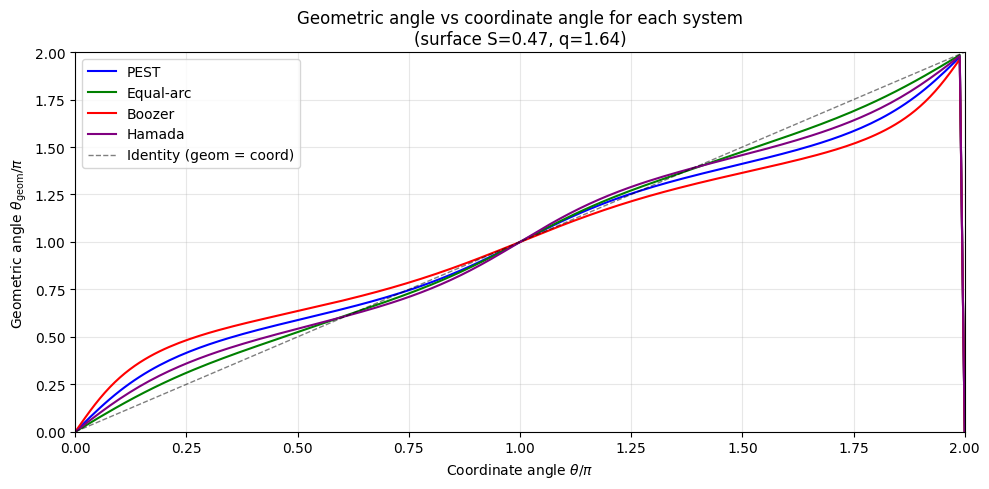
All four systems differ only in how θ is distributed around the flux surface.